

1. Introduction
Aluminum alloy is one of the key materials in modern industries because of its high specific strength, good corrosion resistance and formability [1]. Keyhole laser welding has been widely used as a high-efficient approach to achieve high-integrity joining of aluminum alloy structure. Keyhole laser welding has many advantages, such as high power density, low heat input, high penetration and narrow heat affected zone. In particular, the weldability of aluminum alloy (typical high reflectivity material for infrared laser) can be greatly improved through keyhole welding [2,3]. In keyhole laser welding, the power density of the focused laser beam can reach as high as 1010-1012 W/m2 [4]. At such high power density, metal irradiated by the laser will evaporate instantaneously and form the so-called “keyhole” [5]. During laser welding, the existence of keyhole and its complex interaction with the melt in weld pool make the heat transfer and fluid flow highly complicated. The solidification microstructure, which finally determines the performance of joint, is strongly associated with the heat transfer and fluid flow. Therefore, understanding the dynamic behavior of heat and fluid in the molten pool, and their effects on the solidification microstructure in laser welding are of great significance for performance improvement.
With recent advances in computational power, computational fluid dynamics (CFD) method has been widely used to study the heat transfer and fluid flow during laser welding. Rai et al. [5,6] developed a rigorous, computationally efficient model for keyhole laser welding of various materials, including aluminum, titanium, stainless steel, vanadium, etc. The temperature fields and the fluid flow patterns were predicted, and validated by comparing the simulated weld cross-sections with the experiments. Cho and Na [8] simulated the keyhole formation during laser welding with a novel numerical model, in which multiple reflections and Fresnel absorption were implemented simultaneously with the proposed ray tracing technique. Based on this model, they studied the molten pool dynamics in high power disk laser welding [9]. The calculated fusion zone profile was in good agreement with the experimental result. Pang et al. [10] proposed a three-dimensional (3D) sharp interface model to investigate the self-consistent keyhole and weld pool dynamics in deep penetration laser welding. Furthermore, they extended the model to study the keyhole and weld pool dynamics in tandem dual beam laser welding [11], and in laser welding under variable ambient pressure [12]. Li et al. [13] developed a 3D numerical model to study the keyhole dynamic and melt flow during laser welding of 5A86 aluminum alloy under subatmospheric pressures. Above literatures are mostly focused on partial penetration welding. On the other hand, there are several researches focused on the full-penetration laser welding. Zhao and DebRoy [14] developed a numerical model to predict the keyhole geometry and temperature profiles during full-penetration laser welding. The calculated weld pool dimensions under different welding speeds agreed well with the experimental results. Bachmann et al. [15] developed a 3D steady-state numerical model to study the weld pool dynamics during high-power full-penetration laser welding. Particularly, the effects of the alternating current magnetic field were considered in the model. Panwisawas et al. [16] developed a physics-based 3D model for full-penetration laser welding of Ti-6Al-4 V titanium alloy. The model was able to predict the weld pool geometry and temperature history. Overall, previous works have illustrated that CFD simulations are capable of describing the heat transfer and fluid flow in keyhole laser welding.
The performance of the weld is primarily affected by the solidification microstructure, which depends on the thermal and convective behavior during welding [17]. Although experimental works have depicted the final solidification microstructure by metallographic observation or electron back-scattered diffraction, it is difficult to understand and predict the solidification behavior due to the transient and spatial variations during solidification in welding. For alloys undergoing dendritic solidification, previous researches have shown that the morphology and scale of the microstructure for a specific alloy are correlated with the solidification parameters, such as the temperature gradients, the solidification rate and their combined forms [[17], [18], [19], [20]]. Based on these theoretical understandings, much work has been done to understand the relationship among processing parameters, solidification parameters and solidification microstructure in welding and metal additive manufacturing. Hagenlocher et al. [21] proposed an explicit analytical model to study the effect of laser welding parameters on the grain structure in aluminum alloy welds. The model linked the solution of the 2D heat conduction equation with the solidification parameters and hence the solidification structure map. The model was tested using the AA6016 aluminum alloy. Metallographic analyses proved that the model can well predict the grain structure of laser welds. Rai et al. [6] calculated the solidification parameters during partial-penetration laser welding of 5754 aluminum and 304 L stainless steel by a computationally efficient convective heat transfer model. They pointed out that plane front solidification criterion was not satisfied for both alloys in the examined conditions. It was further found that the solidification structures became coarser and less dendritic as the welding speed decreased. Furthermore, they extended their model for partial and full penetration keyhole laser welding of thick A131 structural steel [22]. They found that the weld microstructure became coarser with the increase in heat input, by either increasing laser power or decreasing welding velocity. Wei et al. [23,24] studied the crystal growth during welding considering the motion of the melt pool. The temperature distribution and the solidification parameters were combined with the grain growth model in a computationally efficient manner. The computed results were tested against independent experimental data. Ou et al. [25] calculated the solidification parameters and predicted the solidification microstructure via a 3D heat transfer and fluid flow model for wire arc additive manufacturing. Gan et al. [26] modeled the thermal behavior and mass transport in multi-layer additive manufacturing of Ni-based alloy on cast iron based on a 3D CFD model. They found that the cooling rate decreased gradually as the subsequent layers deposit, leading to the solidification microstructure getting coarser in the upper part. It can be concluded that combining the simulated temperature data and the solidification parameters can provide a practical way for predicting the solidification microstructure in welding.
From the literature mentioned above, considerable research has been devoted to the partial penetration laser welding or additive manufacturing process. Although several researchers have paid attention to the full-penetration laser welding, related studies are still limited so far. Especially, the heat transfer and fluid flow and their effects on solidification microstructures are not well understood for the full-penetration laser welding of thin aluminum alloy sheet. The present work aims to investigate the heat transfer and fluid flow, and their effects on the morphology and scale of solidification microstructure in full-penetration laser welding of aluminum alloy sheet. This work can provide a theoretical basis for microstructure optimization in full-penetration laser welding of aluminum alloy sheet. The rest of the paper is summarized as follows: In Section 2, the experimental details are described. The description of the numerical model, including governing equations, free surface tracking method, heat source, boundary conditions and numerical implementations, is provided in Section 3. In section 4, the numerical model is first validated by experiments. Then, the heat transfer and fluid flow, and their effects on solidification parameters and solidification structure during welding are discussed. Finally, the conclusions are given in Section 5.
2. Experimental details
The 1.0 mm thickness 5083 aluminum plate was selected as the base material. The 5083 Al alloy is widely used for many applications in automotive, marine and construction industries due to its high strength-to-weight ratio, excellent corrosion resistance, and toughness [27]. The chemical composition was Al-0.20Si-0.08Cu-4.5 Mg-0.18Zn-0.50Mn-0.10Ti-0.10Cr-0.08Fe in weight percent. The laser welding system is shown in Fig. 1. The fiber laser welding experiments were conducted using a continuous wave fiber laser (IPG YLR-4000) with a maximum power of 4 kW. The wavelength was 1.07 μm and the spot diameter was 0.4 mm at the focal position. The defocus distance was 0 mm. The base metal plates were machined to 200 mm × 100 mm × 1 mm, and cleaned carefully by acetone to remove possible oil stain and the oxide film. During laser welding, a high-speed CMOS camera (Phantom v611, America) was used to monitor the dynamic behavior of the weld pool with a photographing speed of 2000 frame per second (fps). The 10 W diode laser with 808 nm wavelength was used to illuminate the weld zone. A narrow band-pass (808 ± 3 nm) interference filter was installed in front of the camera lens to improve the contrast between the weld pool and other regions. Before welding, a calibrated scale was placed at the observation location, and photos were taken by the camera. Using these photos, the relationship between the length in the real world and the length in photos can be established.
Fig. 1.
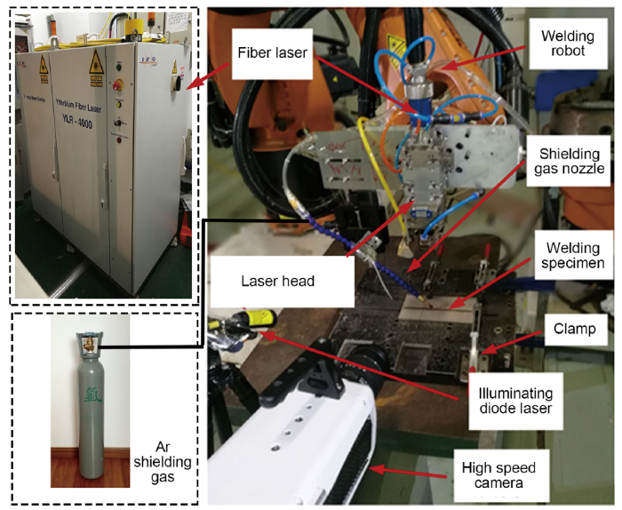
Fig. 1.
Laser welding system.
After welding, the welds were cut, ground, polished, and etched by Keller’s reagent (2.5 mL HNO3 + 1.5 mL HCl + 1.0 mL HF + 95 mL H2O). The weld dimensions were measured by a stereoscopic microscope, and microstructure was observed using a scanning electronic microscope (SEM). For the electron back-scatter diffraction (EBSD) tests, samples were firstly polished by the standard metallographic method, and then electropolished in 10 % perchloric acid and 90 % ethyl alcohol at room temperature and a voltage of 20 V for 15 s. The EBSD tests were carried out on a scanning electron microscope (TESCAN MAIA3) equipped with an HKL-EBSD system. The EBSD data were analyzed by an orientation imaging microscopy (OIM) software.
3. Numerical modeling
3.1. Governing equations
Keyhole laser welding process involves a variety of complicated physical phenomena, such as heat transfer, fluid flow, and phase interaction. The schematic of the full-penetration laser welding of aluminum sheet is shown in Fig. 2. To make the model tractable, the following assumptions were made [28]: (1) The molten metal was laminar and incompressible Newtonian fluid; (2) The material was isotropic homogeneous; (3) Permeation was out of consideration among different phases; (4) The flow of metal vapor was ignored; (5) The beam energy was modeled as a volumetric heat source. The governing equations for simulating heat transfer and fluid flow in 3D Cartesian coordinate are described as follows [29].
Fig. 2.

Fig. 2.
Schematic of the full-penetration laser welding of aluminum sheet.
Continuity equation:
where ρ is fluid density, t is time, V is the velocity vector.
Momentum equation:
where P is the static pressure, g is gravitational acceleration, Cmushy is the mushy zone constant (a value of 1.6 × 10⁴ was used in the present study [6,30]), A is a small computational number introduced to avoid division by zero. FM is the force source term. The third term on the right hand of Eq. (2) is the momentum sink due to the reduced porosity in the mushy zone. μ is the dynamic viscosity which is set as a very large number in solid, a small constant in liquid, and a function of liquid fraction in the mushy zone expressed as follows [31]:
Energy equation:
where h is the enthalpy, λ is the thermal conductivity, SE is the energy source term. The enthalpy considering the solid-liquid phase transition is formulated as [33]:
where Cp,s and Cp,l are the specific heat of solid and liquid, respectively. Lf is the latent heat of fusion.
3.2. Free surface tracking method
The liquid-gas free surface is tracked by the volume of fluid (VOF) method. The temporal evolution of volume fraction (F) can be described as [29]:
According to the definition, F = 1 when a cell is full of liquid, whereas F = 0 when a cell is full of gas. A cell with 0 < F <1 is on the free surface of liquid and gas.
3.3. Laser heat source
with
where P is the laser power, ηl is the effective absorption coefficient, Q0 is the power density at the central axis, ze and zi(t) are the z coordinate of the top surface and bottom surface of heat source, respectively. Note that the x-axis is along the welding direction, y-axis is along width direction, and z-axis is along the vertical depth direction. zi(t) is related to the keyhole depth and is time-dependent. re and ri are the effective radii of heat source at ze and zi(t), respectively. χ is a proportion factor to describe the difference between the peak power densities at ze and zi(t). q(r, z) is considered as an energy source term SE in the energy equation, i.e., Eq. (5).
3.4. Boundary conditions
Fig. 3 illustrates the schematic of the computational domain. Three subdomains are included, i.e., the aluminum domain, the upper gas domain, and the lower gas domain. The two gas domains allow for the free surface deformation during welding. The boundary conditions for the computational domain are described as follows.
Fig. 3.
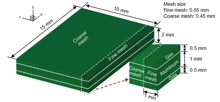
Fig. 3.
Schematic of the computational domain.
3.4.1. Energy boundary conditions
The top surface and bottom surface of the computational domain are set as pressure outlet and ambient temperature. The front domain surface is set as symmetric boundary to reduce the computational cost. Other domain surfaces are treated as wall boundary including heat convection and radiation. The thermal boundary of the wall is described as follows [29]:
where T and T0 are workpiece temperature and ambient temperature, respectively; ε is surface radiation emissivity; σ is Stefan-Boltzmann constant; hconv is convection coefficient.
For the liquid-gas free surface, by considering heat convection, heat radiation as well as liquid evaporation, the thermal boundary conditions can be expressed as [29]:
with
where ΔH* is the enthalpy of vapor flowing at sonic velocity, M is the atomic mass, R is the universal gas constant, TLV is the equilibrium temperature between gas and liquid, ΔHLV is the latent heat of evaporation, and γc is a proportionality factor. Note that the thermal boundary conditions on the liquid-gas interface are implemented via adding the energy source term SE in the energy equation, i.e., Eq. (5).
3.4.2. Driving forces
Cells situated on the liquid-gas free surface are subjected to several pressures, including hydrostatic pressure, hydrodynamic pressure, recoil pressure, and pressure caused by surface tension. The hydrostatic pressure and hydrodynamic pressure are implicitly solved in the momentum equation. The other two pressures on the free surface can be described as:
where Pγ is the pressure which results from the surface tension, Pr is the recoil pressure.
Pγ is formulated as [35]:
with
where γ is the surface tension coefficient, κ is the free surface curvature, γ0 is the surface tension at the melting point Tl, dγ/dT is the surface tension gradient, and n $\vec{n}$ is the unit normal vector of the free surface. It should be noted that the effects of surface tension at the free surface are modeled by the continuum surface stress (CSS) method [36], which results in a source term FM ${{\vec{F}}_{M}}$ in the momentum equation.
The recoil pressure induced by the evaporation process can be given by [37]:
where P0 is the atmospheric pressure. Pr result in a source term FM ${{\vec{F}}_{M}}$ in the momentum equation.
3.5. Numerical implementations
The numerical model is solved by the finite volume method. The simulations were performed using the commercial CFD software ANSYS 18.0/Fluent. The Pressure-Implicit with Splitting of Operators (PISOs) pressure-velocity coupling method [38] was adopted to solve the governing equations with the boundary conditions. The user-defined functions (UDF) written in C language were used to add the energy source terms (Eqs. (8) and (11)) and the force source term (Eq. (18)) to the corresponding governing equations. The surface tension (Eq. (15)) was implemented through the built-in CSS model in the phase interaction module of Fluent.
The thermo-physical properties of 5083 aluminum alloy are listed in Table 1 [39,40]. The heat source parameters are tabulated in Table 2 [41,42]. The configuration of the solution domain is shown in Fig. 3. The solution domain was set as 15 mm in length, 10 mm in width, and 2 mm in depth. Note three subdomains were included with 1 mm height of aluminum domain, 0.5 mm height of gas domain upper the aluminum domain, and 0.5 mm height of gas domain below the aluminum domain. The fine cell with a size of 0.05 mm was used in the weld pool region (1 mm width) where both heat transfer and fluid flow occur. The coarse cell with a size of 0.45 mm was used outside of the weld pool region where only heat transfer occurs. The time step was set as 2 × 10⁻⁵ s. Convergence criterions were 1 × 10⁻⁶ for energy equation and 1 × 10⁻³ for other equations. All the simulations were performed on a workstation with two Intel(R) Xeon(R) E5-2697 v3 @2.60 GHz. Parallel computation with 16 processes was employed to accelerate the simulations using the message passing interface (MPI) library. For all simulations, the length of simulated welding seam was around 10 mm. The computational time ranged from 30 h to 60 h for different welding cases.
| Physical properties | Value |
|---|---|
| Density of liquid (Dl) | 2380 kg/m3 |
| Density of solid (Ds) | 2660 kg/m3 |
| Viscosity (μ) | 1.2 × 10⁻³ kg/m s |
| Specific heat of liquid (Cp,l) | 1198 J/kg K |
| Specific heat of solid (Cp,s) | 1150 J/kg K |
| Latent heat of fusion (Lf) | 3.87 × 10⁵ J/kg |
| Thermal conductivity of liquid (λl) | 90 W/m K |
| Thermal conductivity of solid (λs) | 120 W/m K |
| Liquidus temperature (Tl) | 911 K |
| Solidus temperature (Ts) | 864 K |
| Heat transfer coefficient (hconv) | 20 W/m2 K |
| radiation emissivity | 0.3 |
| Surface tension (γ0) | 0.871 N/m |
| Surface tension gradient (dγ/dT) | -0.155 × 10⁻³ N/m K |
Table 2 Parameters of heat source.
4. Results and discussion
4.1. Grid size independence and time step study
To validate the grid size independence of the simulations, two sets of simulations with different grid sizes of 0.05 mm and 0.025 mm at the fusion zone region were conducted (laser power 2500 W, defocus distance 0 mm, and welding velocity 80 mm/s). The time step was 2 × 10⁻⁵ s. The temporal temperature variations at one point, 0.5 mm away from the centerline, on the mid-depth horizontal plane are displayed in Fig. 4. It is clear that the temperature variations with different grid sizes are almost the same. On the other hand, the influence of time step on the convergence behavior was studied under the welding condition mentioned above. The time step was set as 1 × 10⁻⁵ s and 2 × 10⁻⁵ s, respectively. The grid size at the fusion zone region was 0.05 mm. The temporal variations of temperature are nearly the same as can be seen in Fig. 4. In the following numerical simulations, the grid size and time step are set as 0.05 mm and 2 × 10⁻⁵ s, respectively.
Fig. 4.
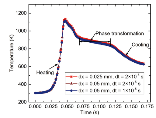
Fig. 4.
Temperature variation with time at one point (0.5 mm away from the centerline) at the mid-depth horizontal plane using different grid sizes and time steps.
4.2. Model validation
The numerical model was validated by comparing with the corresponding experimental results from two aspects. Three series of welding experiments were conducted, and compared in the present study. For all three experiments, the defocus distance was 0 mm. Other welding parameters including laser power (PL) and welding velocity (V) were as follows: Case I PL = 2500 W, V = 80 mm/s; Case II PL = 3000 W, V = 120 mm/s; Case III PL = 3500 W, V = 180 mm/s. Note that these welding parameters were chosen in the premise of the acceptable weld formation after several trials. The first comparison is the weld cross-section profile, which is a common way for validating the simulation results [6]. As displayed in Fig. 5, the white dashed line indicates the experimental weld profile, and the red dashed line represents the simulated weld profile. Because no single cross-section of weld geometry represents the fusion zone cross-section, the simulated weld profile was obtained by taking the projection of the computed three-dimensional solidus contours on the transverse plane (projective plane). It can be seen that the experimental and simulated weld profiles are in good agreements overall. The second comparison is the morphologies of the top surface of weld pool. Fig. 6(a), (c) and (e) show the experimental high-speed camera images of the weld pool top surface for three welding cases. Because of the low contrast between the molten metal and the solid metal, it is hard to identify the weld pool boundary directly. Alternatively, the weld pool boundary can be recognized due to the fluctuation of molten metal. The morphology of the weld pool free surface varies with time because of the movement of molten metal. The weld pool boundary can be identified according to the difference of two successive frames. In Fig. 6(a), (c) and (e), the upper image shows the weld top surface at reference time t, and the lower image (the following frame after the upper image) displays the weld top surface at time t +0.5 ms. The dimensions of the weld pool can be estimated according to the calibrated scale at the top-right corner of the figure. Note that the length parallel to the welding direction and the length perpendicular to the welding direction are not equal in the photos due to the perspective view of the camera. It can be seen that the length of weld pool increases significantly from 4.2 mm to 4.7 mm and 5.4 mm. Fig. 6(b), (d) and (f) display the simulated weld pool morphologies. It is worth mentioning that the weld pool profile is indicated by the isothermal of liquidus temperature - i.e., 911 K. As can be seen, the length of weld pool agrees well with the experiments. Overall, the above comparisons manifest the validity of the proposed numerical model, which is capable to investigate the heat transfer and fluid flow in laser welding.
Fig. 5.
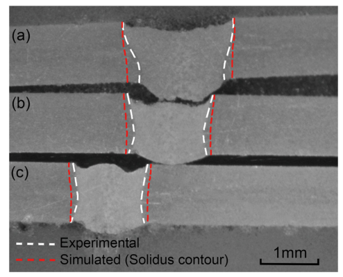
Fig. 5.
Comparison of the experimental and predicted weld cross-section profile: (a) PL = 2500 W, V = 80 mm/s; (b) PL = 3000 W, V = 120 mm/s; (c) PL = 3500 W, V = 180 mm/s.
Fig. 6.
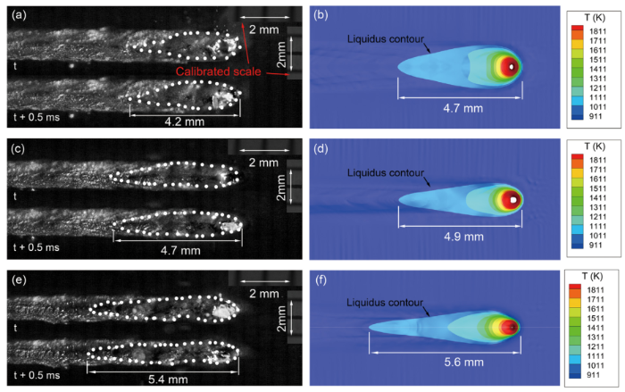
Fig. 6.
Comparison of the top surface morphologies of weld pool between the experimental high-speed camera images and numerical simulations. (a) Experimental: PL = 2500 W, V = 80 mm/s; (b) Simulated: PL = 2500 W, V = 80 mm/s; (c) Experimental: PL = 3000 W, V = 120 mm/s; (d) Simulated: PL = 3000 W, V = 120 mm/s; (e) Experimental: PL = 3500 W, V = 180 mm/s; (f) Simulated: PL = 3500 W, V = 180 mm/s. Note that the weld pool profile in high-speed camera images can be recognized by the fluctuation of molten metal.
4.3. Fluid flow and heat transfer
Fig. 7(a) shows the calculated 3D temperature and velocity fields for Case I with PL = 2500 W and V = 80 mm/s. As can be seen, a through keyhole is formed due to the direct irradiation of laser beam. The weld pool is elongated along the opposite direction of the laser beam movement. The mushy zone- - i.e., the two-phase region containing both the liquid and solid material, is bounded by the liquidus temperature (911 K) and solidus temperature (864 K). The velocity field of molten metal is indicated by the arrows whose magnitude can be estimated by comparing their lengths with the reference vector (1 m/s).
Fig. 7.
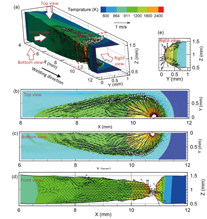
Fig. 7.
Calculated temperature and velocity fields for Case I (PL = 2500 W and V = 80 mm/s) observed from different views: (a) 3D view, (b) top view, (c) bottom view, (d) front view, and (e) right view of section A in a.
Fig. 7(b) and (c) display the top view and bottom view of calculated temperature and velocity fields, respectively. A typical V-shaped tail of the melt contour is observed, which is caused by the latent heat of the solid-liquid phase transition [43]. The temperature of the molten metal at the keyhole surface reaches the boiling point while molten metal at the weld pool boundary remains at the liquidus temperature. A temperature gradient is set up at both the top and bottom weld pool surfaces. Note that the surface tension (γ) of molten metal declines significantly as temperature (T) increases (∂γ/∂T < 0). Therefore, a significant spatial variation of the interfacial tension is induced at the surface of weld pool. Marangoni convection occurs due to the surface tension gradient along the weld pool surface. As a result, the molten metal moves radially outward around the keyhole at both the top surface (Fig. 7(b)) and the bottom surface (Fig. 7(c)). Fig. 8 shows the temperature distribution along the weld centerline. It can be seen that the temperature gradient is extremely sharp near the keyhole, and becomes flat away from the keyhole. The larger the temperature gradient is, the stronger the Marangoni convection tends to be. Therefore, strong Marangoni convection can be observed near the keyhole region where high temperature gradient appears in Fig. 7(b) and (c). By contrast, the Marangoni effect is weak at the rear of weld pool away from the keyhole since the temperature gradient is low. In addition, it can be observed that the molten metal flows backward to the rear part along the weld pool boundary and returns through the weld center, which makes a circulation loop develop at the rear of weld pool. This flow characteristic is consistent with Chang’s simulation result about full-penetration laser welding of titanium alloy plate in 3 mm thickness [44]. Fig. 7(d) shows the temperature and velocity fields at the symmetry plane in Fig. 7(a) from the front view. There exist two evident circulation loops induced by Marangoni force ahead of the keyhole. Behind the keyhole, two obscure circulation loops caused by the Marangoni effect can be observed at the front of weld pool. At the rear of weld pool, the molten metal flows forwards to the keyhole, and no significant Marangoni flow loop is observed due to the very low temperature gradient. Fig. 7(e) shows the temperature and velocity profiles at section A in Fig. 7(a) from the right view. Similar to the flow characteristic ahead of the keyhole in Fig. 7(d), two obvious circulation loops induced by the Marangoni effect dominate the weld pool.
Fig. 8.
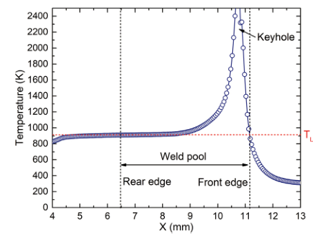
Fig. 8.
Temperature distribution along weld centerline for Case I (PL = 2500 W and V = 80 mm/s).
where u is the characteristic fluid velocity, ρ is the density, Cp is the specific heat, LR is the characteristic length, and λ is the thermal conductivity. The contribution of convection to heat transfer increases with the increase of Pe. It is worth mentioning that the Pe varies with the location within the weld pool. The high-velocity region near the weld pool surface will have a higher Pe compared with the low-velocity region inside the weld pool. Even in systems where heat conduction is the dominant mechanism of heat transfer, the Pe near the weld pool surface will be high due to the large local fluid velocities. Considering a typical velocity of 100 mm/s, a characteristic length of 0.8 mm (half width of the weld pool), and the properties of the liquid metal, the calculated Pe works out to be about 1.9, which is consistent with the calculated value (about 2.0) for partial penetration laser welding of 5754 aluminum alloy in Ref. [6]. The low Pe indicates that heat conduction plays a dominant role in heat transfer in the weld pool. This can be intuitively understood from the temperature contours and flow patterns in the weld pool. As shown in Fig. 7, the temperature contours do not strictly follow the recirculating flow pattern since significant heat transfer takes place by heat conduction. This is significantly different from laser welding of stainless steel and titanium, where convection is the main mechanism of heat transfer [6,7].
4.4. Effects of welding parameters
The laser power (PL) and welding speed (V) are two of the most influential and easily controllable parameters in laser welding. As mentioned previously, three welding cases with an appropriate match between PL and V were conducted. The laser power increases from 2500 W to 3000 W and 3500 W, and the welding speed increases correspondingly from 80 mm/s to 120 mm/s and 180 mm/s. The calculated 3D temperature and velocity fields for three welding cases are shown in Fig. 9. It can be seen that there is no obvious difference in the flow pattern and velocity magnitude among three cases. However, the predicted weld width decreases significantly from Case I to Case III, which shows the same trend with experiments (Fig. 5). This can be attributed to the decrease in net heat input, which is defined as the heat input per unit length, i.e. ηlPL/V. From Case I to Case III, the net heat input decreases from 21.88 J/mm to 17.50 J/mm and 13.61 J/mm. In addition, the weld pool and mushy zone tend to become more elongated from Case I to Case III as shown in Fig. 9(a), (b) and (c). This tendency agrees well with Aalderink et al.’s work, in which the effects of welding parameters on the weld pool geometries in laser welding of thin sheets of AA5182 aluminum alloy were investigated via a 2D finite element multi-physical model [45]. Note that the mushy zone is the two-phase solid-liquid region located between the solidus contour (864 K) and liquidus contour (911 K). With the variation of welding parameters, the mushy zone geometry is affected by two opposing factors. First, the mushy zone may become elongated with the increase in welding speed. Second, an increase in welding speed and the decrease in the net heat input per unit length may reduce the mushy zone size. Which of these two opposing factors will dominate depends on the material properties like thermal conductivity and specific heat, and process parameters like welding speed and heat input. It is expected that the former effect will dominate till very high welding speed for materials with high thermal diffusivity [6]. Therefore, the mushy zone becomes more elongated from Case I to Case III since aluminum alloy has high thermal conductivity. The size of the mushy zone has a significant influence on the solidification parameters and the grain morphologies during solidification.
Fig. 9.
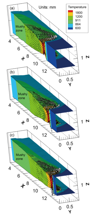
Fig. 9.
Calculated temperature and velocity fields for different welding parameters: (a) PL = 2500 W, V = 80 mm/s; (b) PL = 3000 W, V = 120 mm/s; (c) PL = 3500 W, V = 180 mm/s.
4.5. Solidification parameters and grain/sub-grain structures
Solidification structure in laser weld is significantly influenced by the thermal behavior. Two key parameters, temperature gradient G and solidification rate R, affect the microstructure formation at the liquid-solid interface. G and R can be expressed as follows:
where n $\vec{n}$ is the unit normal vector of the liquid-solid interface, and i $\vec{i}$ represents the unit vector of the welding direction. The solidification morphology and the microstructure scale are determined by the combined forms of G and R. While their product GR (representing the cooling rate), determines the scale of microstructure, their ratio G/R is linked to the morphology of solidified microstructure [17]. The effect of G and R on the morphology and size of solidification microstructure is illustrated in Fig. 10 [15].
Fig. 10.

Fig. 10.
Schematic diagram illustrating the effect of temperature gradient G and growth rate R on the morphology and size of solidification microstructure [15].
Fig. 11 displays the variation of G and R as a function of weld width at the mid-depth horizontal plane with PL = 2500 W and V = 80 mm/s. Note that the heat flow during welding can be regarded as two-dimensional in this work since the temperature distribution is almost the same along thickness direction as can be seen from Fig. 7, Fig. 9. The solidified microstructure is considered to be identical throughout the weld thickness. Therefore, the variation of solidification parameters and solidified microstructure at the mid-depth horizontal plane can represent those of the whole weld. The shape of the molten pool is displayed to help understand the influence of the liquid-solid interface profile on G and R. As the model is at the continuum-scale, individual dendrites are not simulated. G and R are approximated from the isothermal T = (TL + TS)/2 = 887.5 K, where TL and TS are the liquidus temperature and solidus temperature, respectively. In Fig. 11, the relationship between the solidification direction n and the slope of the isothermal contour (887.5 K) is illustrated. A more horizontal slope of liquidus results in a lower R because the normal of the isothermal contour is misaligned to the welding direction. As the normal of liquidus contour is perpendicular to welding direction at the fusion boundary, R becomes almost zero. By contrast, R increases to the welding speed when the normal of liquidus is parallel to the welding direction. On the other hand, the distance between the liquidus and solidus can be used to discern the variation of G. As shown in Fig. 11, G decreases dramatically from the fusion boundary to the centerline. G is approximately 350 K/mm at the fusion boundary, whereas it is only about 20 K/mm at the weld centerline. On the contrary, R increases significantly from nearly 0 mm/s to 80 mm/s from the fusion boundary to the centerline.
Fig. 11.
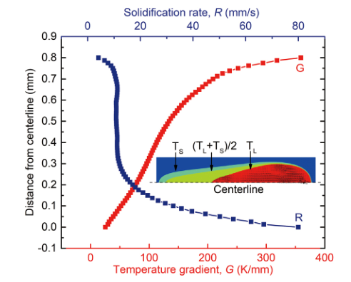
Fig. 11.
The spatial variation of the temperature gradient G and solidification rate R along the representative isothermal (TL + TS)/2 in the mushy zone as a function of weld width at the mid-depth horizontal plane. The welding parameters are PL = 2500 W and V = 80 mm/s.
Fig. 12(a) and (b) compare the variation of G and R along the representative isothermal (887.5 K) in the mushy zone for three different welding cases. The spatial variations of G and R leads to the change in solidification parameters, which have a significant influence on the morphology and scale of microstructure. The morphology factor G/R determines the solidification morphology (Fig. 10). High G/R values indicate the solidification propagates stably as a planar front, while low G/R values indicate it grows unstable as cellular or dendritic structures [17]. The constitutional supercooling criterion states that stable planar solidification will proceed if the following condition is satisfied:
where ΔTeq is the range of equilibrium freezing temperature (22 K for 5083 aluminum) and DL is the solute diffusion coefficient (3 × 10⁻³ mm2 s-1 for Mg in liquid Al [46,47]). Thus, the calculated value of ΔTeq/DL for 5083 aluminum is approximately 7 × 10³ K s/mm2. Fig. 12(c) shows the variation of G/R along the solid/liquid interface in three different cases. For all three cases, the G/R values decrease greatly from the fusion boundary to the centerline. All these values are significantly lower than the critical value of 7 × 10³ K s/mm2. Therefore, cellular or dendritic solidification structure is expected to form in the welds, which is well consistent with the SEM observations in the following.
Fig. 12.
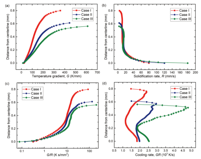
Fig. 12.
Comparison of the solidification parameters along the representative isothermal (887.5 K) in mushy zone for different welding cases: (a) temperature gradient G, (b) solidification rate R, (c) morphology factor G/R, (d) cooling rate GR. The welding parameters are: Case I - PL = 2500 W, V = 80 mm/s; Case II - PL = 3000 W, V = 120 mm/s; Case III - PL = 3500 W, V = 180 mm/s.
where d is the secondary dendrite arm spacing (SDAS); ε is the cooling rate, which is equal to GR here; n is between 0.33 and 0.5; a is a fitting factor, which depends upon the alloy elemental concentration and constituents. Fig. 12(d) shows the derived cooling rate GR along the solid/liquid interface for three welding cases. Overall, the cooling rate increases from Case I to Case III due to the decline in heat input. For all three cases, GR firstly increases sharply, then decreases gradually, and finally increases slowly from the fusion boundary to the centerline. GR around the weld centerline increases from about 1750 K/s to 1950 K/s and 2650 K/s from Case I to Case III. Fig. 13(a), (b) and (c) display the SEM images around the centerline of the laser welds for three cases, from which dendritic solidification structures can be observed obviously. This is in good consistency with the above morphology prediction by G/R values. Furthermore, the microstructure scale is evaluated by SDAS. To determine SDAS, the total spacing from the first to the last arm needs to be measured (well developed and parallel dendrite arms in the micrograph should be selected). Then it is divided by the number of existing dendrite arms in this area. After repeated measurements in different areas, the average value of the results and its scattering are calculated. As the cooling rate increases, SDAS decreases significantly from 4.1 μm to 3.9 μm and 3.4 μm. On the other hand, the dendritic solidification structures are simulated using the quantitative phase-field model for alloy solidification. Details of the model can refer to [43,44]. In the simulations, the base metal is assumed as a dilute binary Al-4.5 Mg alloy. The simulated results under three different cooling rates are shown in Fig. 13(d) (e) and (f). As can be observed, the dendritic structure becomes finer as the cooling rate increases, which is consistent with the experimental results. However, the measured SDAS are 3.3 μm, 3.1 μm, and 2.9 μm, respectively, all of which are slightly smaller than the corresponding experimental results. Fig. 14(a) plots the SDAS obtained from experiments and phase-field simulations, as well as the fitted curves according to Eq. (23). The corresponding fitted values of a and n are displayed in Fig. 14(b). The fitted values of a and n from phase-field simulations are 41.35 μm and 0.339, which are similar to the values (a =55.9 μm, n = 0.34) fitted by Easton et al. [48]. Especially, a good agreement of the value of n is observed. However, the fitted values of a and n from the experiments are 118.53 μm and 0.451, which are considerably different from the values fitted from phase-field simulated results and the values fitted by Easton et al. [45]. The discrepancy in n value can be attributed to the melt convection in the weld pool. Theoretical models have shown that the values of SDAS and n tend to increase when including the solute redistribution by both the convective and diffusive means [49]. This has been verified by experiments in which forced convection was produced by the magnetic field. It was found that the melt convection can increase the coarsening rate of secondary arms, which leads to an increase in SDAS and tends to give an n value closer to 0.5 [50]. On the other hand, this can explain why the phase-filed simulated SDAS (without considering the melt convection) is smaller than the experimental results (convection may play an important role).
Fig. 13.

Fig. 13.
The dendritic structures and their microstructure scale under various cooling rate in three welding cases: (a) (c) Case I - PL = 2500 W, V = 80 mm/s; (b) (e) Case II - PL = 3000 W, V = 120 mm/s; (c) (f) Case III - PL = 3500 W, V = 180 mm/s. (a), (b) and (c) are experimental results tested by SEM; (d) (e) and (f) are phase-field simulated results colored by the Mg content.
Fig. 14.
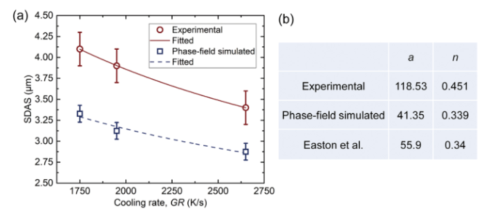
Fig. 14.
(a) SDAS obtained from experiments and phase-field simulations under different cooling rates, and the corresponding fitted curves based on Eq. (23); (b) comparison of the fitted a and n among the experimental results, the phase-field simulated results, and Easton et al.’s experimental results [45].
In laser welds, it is possible to have either columnar grains (growing epitaxially from fusion line) or equiaxed grains (nucleating ahead of the solidification front). The behavior of columnar to equiaxed transition (CET) has been well investigated in previous work [51,52], so only the final expression is given here. The relationship among the volume fraction of equiaxed grains ϕ, the primary solidification parameters, and the material-dependent parameters is described as [52]:
where a and n are the material dependent parameters, N0 is the number of nucleation sites. It is worth noting that the parameters a and n are related to the constitutional tip undercooling for columnar and equiaxed dendritic growth, which satisfies ΔT = (aV)1/n with the undercooling ΔT and the dendrite growth rate V. Hunt [51] proposed that ϕ > 0.49 can be considered as fully equiaxed growth. Thus, the grain structure in the weld can be predicted by calculating the critical values of Gn/V. For simplicity, the dendrite growth rate V is approximated to the solidification rate R. According to Greer [53], the material-dependent constant is derived as n = 3 and a = 6.19 K3 m/s. It should be noted the number of nucleation sites N0 is fitted to be 2.77 × 10¹³ m-3 based on the experimental grain structure of Case I since no relevant data are available for the 5083 aluminum alloy used in this work. Consequently, the condition for fully equiaxed grain formation is derived to be G3/R < 1.66 × 10⁵ K3 s/mm4.
Fig. 15(a), (c) and (e) show the spatial variation of the calculated CET parameter, G3/R, along the solid/liquid interface for different cases. As can be seen, G3/R decreases significantly from a magnitude order of 107 to a magnitude order of 10 from the fusion boundary to the weld centerline, indicating that a transition from columnar to equiaxed grain morphology is possible. The critical value of (G3/R)critical for fully equiaxed grain formation is indicated at the G3/R axis by the black arrow. The region where G3/R < (G3/R)critical is thus the predicted fully equiaxed region, which is actually half width of the equiaxed region of the whole weld. Note the solidification parameters and grain structure in the weld are symmetric about the weld centerline. The corresponding experimental grain structures tested by EBSD are displayed in Fig. 15(b), (d) and (f). Only half of the whole weld is shown here due to the symmetry, with the weld centerline at the bottom and base metal on the top. It can be seen that columnar grains grow epitaxially from the base metal, and grow competitively with each other to the weld center until they are fully blocked by the equiaxed grains. In the weld, three grain regions exist, namely the fully columnar grain region, the fully equiaxed grain region, and a very small transition region. Here, only the fully equiaxed grain region is predicted, and the remaining region in the weld is simply considered as columnar grain region. In Fig. 15(b), (d) and (f), the fully equiaxed grain region predicted by CET parameter G3/R is located between the dash-dot line (centerline) and dash line (extended from the left figure at the critical G3/R), which is indicated by the double arrowhead line. It can be seen that the predicted results agree well with the experimental results. Both predictions and experiments indicate that the width of the equiaxed region decreases with the decline in net heat input from Case I to Case III. This is primarily because that G3/R increases more and more rapidly from Case I to Case III, which tends to make a larger undercooling zone ahead of the solidification front that promotes the nucleation of equiaxed grains.
Fig. 15.
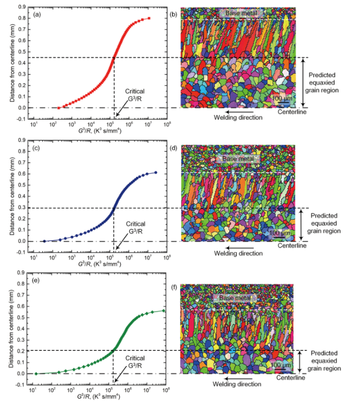
Fig. 15.
Spatial variation of the CET parameter, G3/R, along the representative isothermal (887.5 K) in mushy zone and the corresponding experimental grain structures tested by EBSD for different cases: (a)(b) Case I - PL = 2500 W, V = 80 mm/s; (c)(d) Case II - PL = 3000 W, V = 120 mm/s; (e)(f) Case III - PL = 3500 W, V = 180 mm/s.
5. Conclusions
The heat transfer and fluid flow, and their effects on the solidification microstructure in full-penetration laser welding of 1.0 mm thickness 5083 aluminum sheet are examined in this work. The predicted weld pool dimensions, as well as the microstructure morphology and scale for three different welding cases (laser power: 2500, 3000, 3500 W; welding speed: 80, 120, 180 mm/s) agree well with the corresponding experimental results. The main conclusions can be drawn as follows:
(1) Significant Marangoni convection occurs in the weld pool near the keyhole. Away from the keyhole, the Marangoni effect is weak because of the low temperature gradient.
(2) Heat conduction is the main mechanism of heat transfer inside the weld pool. Melt convection plays a critical role in the microstructure scale (increasing the SDAS).
(3) The mushy zone shape/size and the solidification parameters can be modulated by altering the process parameters and hence the heat input intentionally.
(4) The low G/R values indicate the high instability of plane front solidification and the formation of dendritic structures in the weld pool.
(5) Finer dendritic microstructure can be obtained by increasing GR via adjusting the process parameters and thus the heat input.
(6) The transition from columnar to equiaxed grain morphology is predicted by G3/R. The transition occurs as G3/R is lower than a critical value (material-dependent).
(7) For full-penetration laser welding of thin aluminum alloy sheet, process parameters with a high laser power and a matched rapid welding speed are recommended from the perspectives of the resulting narrower weld and finer microstructure.
Acknowledgements
This research has been supported by the National Natural Science Foundation of China under Grant No. 5181101756, 51861165202 and No. 51721092, the Major Project of Science and Technology Innovation Special for Hubei Province under Grant No. 2018AAA027, the Fundamental Research Funds for the Central Universities, HUST: No. 2018JYCXJJ034 and No. 2019JYCXJJ025, the Postdoctoral Science Foundation of China under Grant No. 2018M632837, and the opening project of State Key Laboratory of Digital Manufacturing Equipment and Technology (HUST) under grant No. DMETKF2018001. Shaoning Geng is supported by the China Scholarship Council as a visiting scholar at the University of Virginia.
Reference

A single-phase problem is solved rather than a multiphase problem for numerical simplicity: and the solution is based on the assumption that the region of gas or plasma can be treated as a void because solid or liquid steel has a greater density level than gas or plasma. The volume-of-fluid method, which can calculate the free surface shape of the keyhole, is used in conjunction with a ray-tracing algorithm to estimate the multiple reflections. Fresnel's reflection model is simplified by the Hagen-Rubens relation for handling a laser beam interaction with materials. Factors considered in the simulations include buoyancy force. Marangoni force and recoil pressure; furthermore, pore generation is simulated by means of an adiabatic bubble model, which can also lead to the phenomenon of a keyhole collapse. Models of the shear stress on the keyhole surface and of the heat transfer to the molten pool via a plasma plume are introduced in simulations of the weld pool dynamics. Analysis of the temperature profile characteristics of the weld bead and molten pool flow in the molten pool is based on the results of the numerical simulations. The simulation results are used to estimate the weld fusion zone shape; and the results of the simulated fusion zone formation are compared with the results of the experimental fusion zone formation and found to be in good agreement. The effects of laser beam profile (Gaussian vs. measured), vapor shear stress, vapor heat source and sulfur content on the molten pool behavior and fusion zone shape are analyzed. (C) 2011 Elsevier B.V.

 WeChat