aKey Laboratory of Nuclear Materials and Safety Assessment, Institute of Metal Research, Chinese Academy of Sciences, Shenyang 110016, China
bSchool of Materials Science and Engineering, University of Science and Technology of China, Shenyang 110016, China
cShenyang National Laboratory for Materials Science, Institute of Metal Research, Chinese Academy of Sciences, Shenyang 110016, China
Corresponding authors:* Key Laboratory of Nuclear Materials and Safety Assess-ment, Institute of Metal Research, Chinese Academy of Sciences, Shenyang 110016, China.E-mail address:mysun@imr.ac.cn(M.-y. Sun).
Movement and growth of dendrites are common phenomena during solidification. To numerically investigate these phenomena, two-phase flow model is employed to formulate the FSI (fluid-structure interaction) problem during dendritic solidification. In this model, solid is assumed to have huge viscosity to maintain its own shape and an exponential expression is constructed to describe variable viscosity across s-l (solid-liquid) interface. With an effective preconditioner for saddle point structure, we build a N-S (Navier-Stokes) solver robust to tremendous viscosity ratio (as large as 1010) between solid and liquid. Polycrystalline solidification is computed by vector-valued phase field model, which is computationally convenient to handle contact between dendrites. Locations of dendrites are updated by solving advection equations. Orientation change due to dendrite’s rotation has been considered as well. Calculation is accelerated by two-level time stepping scheme, adaptive mesh refinement, and parallel computation. Settlement and growth of a single dendrite and multiple dendrites in Al-Cu alloy were simulated, showing the availability of the provided model to handle anisotropic growth, motion and impingement of dendrites. This study lays foundation to simulate solidification coupled with deformation in the future.
Jian-kun Ren, Yun Chen, Yan-fei Cao, Ming-yue Sun, Bin Xu, Dian-zhong Li. Modeling motion and growth of multiple dendrites during solidification based on vector-valued phase field and two-phase flow models. Journal of Materials Science & Technology[J], 2020, 58(0): 171-187 DOI:10.1016/j.jmst.2020.05.005
1. Introduction
Dendritic growth is a common phenomenon during casting of metals and has a significant impact on microstructure and mechanical property of finished products. As a widely used numerical approach, phase field model can formulate dendritic growth quantitatively and help us better understand the formation of dendritic morphology. Nowadays, it has no difficulty modeling single and polycrystalline dendritic growth of pure metals and alloys, both in 2D and 3D [[1], [2], [3], [4], [5], [6], [7]]. However, lots of previous studies only involved thermal and solute diffusion without melt flow and motion of solids. This is far from the actual situation. To analyze the influence of melt flow on growth, some simulations coupled with fluid dynamics were performed to model fixed dendrite growing in forced or natural convection [[8], [9], [10], [11], [12], [13]]. Nevertheless, these simulations only apply to dendrites attached to mould during casting but not to those moving freely in melt. Consequently, a more realistic model should not ignore movement of solids. There are three issues in the presence of motion of solid.
Firstly, it requires a suitable FSI model to solve flow field both in liquid and solid. Tong et al. [8] forced the velocity in solid to become zero by adding “distributed momentum sink” into momentum equation so that solid couldn’t move at all. Yamaguchi et al. [14,15] employed material point method to model motion, rotation, and even deformation of both single dendrite and polycrystalline structure [14,15]. However, deformation-induced liquid flow was not really solved, but given by “zero-gradient extension”. Consequently, any point in liquid would have the same velocity as the closest solid [14]. LBM (Lattice Boltzmann model) is a promising numerical approach to solve flow problems. Rojas et al. [16,17] employed it to simulate motion and growth of multiple dendrites. In their study, velocity in liquid and each dendrite was solved individually. Total force and torque acting on every dendrite were computed by regarding them as rigid bodies. An alternative is two-phase flow model. Solid is artificially given a viscosity large enough to resist deformation caused by flow [18,19].
Secondly, locations of dendrites should be updated according to computed flow field. This could be accomplished by embedding advection terms into phase field model [14,15,19] directly or solving advection equations individually [16,17].
Thirdly, an appropriate way is necessary to handle orientation evolution of dendrite and its change due to rotation. Otherwise, dendrite might grow into unphysical distorted shapes (Fig. 2(c) in Ref. [14]). Rojas et al. [17] used multiple phase field equations for multiple dendrites and solved them separately. Obviously, more dendrites mean more equations to be solved. A better strategy is to introduce orientation field into phase field model [14,15,19]. In this way, no matter how many dendrites there are, only one phase field variable is required. Treatment of orientation change due to rotation is straightforward according to the rotating rate of dendrite.
Two-phase flow model is our choice to compute flow field. In this approach, two phases can be treated as a whole rather than separately. Different from Refs. [18] and [19] which also chose this approach, we describe dendritic growth by vector-valued phase field model [[20], [21], [22]], which is computationally convenient to handle orientation periodicity (see Section 2.1.2) and collision between solids. Locations of dendrites are updated by solving advection equations individually so that phase field model still leads to symmetric and positive definite stiff matrices. After rigorous numerical tests, we simulated growth, settlement, rotation, and collision of a single dendrite and multiple dendrites in Al-Cu alloy.
The most challenging aspect in this work is the flow field computation with a steep viscosity variation across s-l interface. In this study, two-phase flow is formulated by N-S equations. Unfortunately, lots of studies were focused on huge viscosity jump for Stokes flow [[23], [24], [25], [26]] rather than N-S flow. To ensure numerical stability, an exponential expression is constructed to make the viscosity vary across s-l interface in a relatively steady way. We develop a preconditioner combined with scaling strategy, taking into account the balance between momentum and continuity equation. Two-level time stepping scheme is designed to reduce run time as far as possible (Section 2.4). Adaptive mesh refinement and parallel computation based on MPI protocol are adopted to further accelerate computation. Numerical tests show our model can withstand a tremendous viscosity ratio (1010) between solid and liquid. The numerical approaches we develop to compute flow field in this study would be of great interest in other fields like simulation of the earth’s convective mantle [27], ice sheet [28], and polymer processing techniques [23], which also involve huge viscosity variation. Our code is elaborated based on the finite element library, DEAL.II [48].
2. Model
Symbols in this paper are listed in Appendix D for ease of lookup.
2.1. Phase field model to simulate growth of multiple dendrites
2.1.1. Scalar-valued phase field model
The conventional polycrystalline phase field model takes scalar-valued form and involves following variables: phase field ϕ, temperature T, solute concentration c, and orientation field α [22]. ϕ varies smoothly from -1 in the liquid to 1 in the solid through the diffuse interface. The s-l interface is defined by ϕ = 0. In this study, for pure metal, T is solved and c = 0 all the time; for alloy, T is prescribed as a constant in the whole domain and c is really computed. This is feasible as thermal diffusivity is usually several orders of magnitude larger than solute diffusivity (Section II. in Ref. [3]). α indicates the preferred growth direction of a dendrite (Fig. 1 in Ref. [22]). It ranges from -π/4 to π/4 because cubic metal with 4-fold symmetry is considered in this study. In liquid, α is meaningless but here is set as 0.
The scalar-valued phase field equation reads [15,22]
In the case of pure metal, Eqs. (1), (2), (3) are solved (DT: thermal diffusivity); in the case of alloy, Eqs. (1), (2) and (4) are solved. Solute diffusivity ranges from Dcl in liquid to Dcs in solid. In this paper Dcs = 0 as it’s always several orders of magnitude lower than Dcl [3,29].
In Eq. (1), the diffuse interface thickness W is
$W={{W}_{0}}{{a}_{s}} $
where as (anisotropy) takes the following form in solid:
(ε4: anisotropic strength). (x1, x2) is the location in local frame associated with the orientation of each dendrite (Fig. 1 in Ref. [22]). In liquid, as = 0. W0 (spatial scale) is determined by the ratio W0/d0 (d0: capillary length). This ratio is artificially chosen to facilitate computation in large scale. Coupling constant λ is
$\lambda ={{a}_{1}}\frac{{{W}_{0}}}{{{d}_{0}}} $
(a1 is a constant, see Table 1). Capillary length is
${{d}_{0}}=\left\{ \begin{array}{*{35}{l}} {{d}_{0T}}=\frac{ \Gamma {{c}_{p}}}{L}\left( pure metal \right) \\ {{d}_{0c}}=\frac{ \Gamma }{{{T}_{l-s}}}\left( alloy \right) \\ \end{array} \right. $
where cp and L are the volumetric specific heat and the latent heat. Γ (Gibbs-Thomson coefficient) and Tl-s (freezing range) are
(γ: surface tension, Tm: melting point of solvent, m: liquidus slop, c∞: the initial concentration of the alloy, k: solute partition coefficient). When interface kinetics is negligible in cases like low-speed solidification, for pure metal (Eq. (90) in Ref. [1]) and alloy (Section IV.C.3 in Ref. [3]), the phase field relaxation time is
Fig. 1.
Schematic phase diagram for a typical dilute binary alloy. Blue line: liquidus, red line: solidus. l1 = Tm + mc∞ - T, l2 = Tl-s. cl, cs: equilibrium concentrations in liquid and solid at temperature T.In Eq. (1)
$Y=\left\{ \begin{array}{*{35}{l}} {{U}_{T}}=\frac{T-{{T}_{m}}}{\frac{L}{{{c}_{p}}}}\left( pure metal \right) \\ \theta +k{{U}_{c}}\left( alloy \right) \\ \end{array} \right. $
UT is dimensionless temperature in pure metal, and Uc is dimensionless concentration in alloy:
where s, η, μc, β in Eqs. (1), (2) and (19) are constants given in Table 1.
Homogeneous Neumann boundary conditions are imposed on the whole boundary: N∙∇ϕ, N∙∇α, N∙∇T, N∙∇c = 0. N is the outward unit normal to the boundary. Usually, initial ϕ is given by
where ds is the signed distance from (X1, X2) to s-l interface, with ds < 0 inside and ds > 0 outside the solid respectively. (X1, X2) is location in the global frame (Fig. 1 in Ref. [22]).
2.1.2. Vector-valued phase field model
When dendrites touch each other and grain boundaries begin to form, the orientation periodicity has to be taken into consideration. For example, two grains with α = ±3π/16 should have a misorientation of π/8 (±π/4 represent the same orientation). Without specific treatment, in scalar-valued model, the misorientation would be treated as 3π/8, resulting in incorrect boundary behavior (Fig. 3 in Ref. [22]).
To avoid this, it’s necessary to modify ∇α in Eq. (1) and two additional diffusion equations should be solved (Appendix B.3 in Ref. [2]). This is not easy to implement when finite element method is employed (Section 3.1 in Ref. [22]). Another option to deal with the periodicity is to transform (ϕ, α) into an ordering vector F = (F1, F2) [[20], [21], [22]] (this vector was denoted by “(p, q)” in previous studies [[20], [21], [22]]. In this paper, “p” is the pressure):
which will pose problems during finite element discretization (see Eqs. (A.16)-(A.20) in Ref. [22]), however. To overcome this issue, evolution equations are finally split into (see Ref. [22])
where A1 and A2 stand for the right hand side of Eqs. (1) and (2).
In vector-valued phase field model, during each time step, Eqs. (23) and (24) are solved in turn along the solid line in Fig. 2, followed by Eq. (3) for pure metal or Eq. (4) for alloy. In this study, vector-valued model is adopted to handle the contact between dendrites. Unless otherwise stated, (ϕ, α) shown below is converted from F. Fig. 13(b) gives a view of F distribution near the grain boundary and s-l interface.
Fig. 2.
Evolution of F due to dendritic growth in a time step dt. Dot line: advancing F by equation without splitting (Eq. (22)); solid line: advancing F by “split equation 1” (Eq. (23)) and “split equation 2” (Eq. (24)); F*: intermediate solution.
2.2. Two-phase flow model
In this study, two-phase flow model is used to describe motion of dendrites and flow in melt. Solid is regarded as fluid with extremely large viscosity to have enough resistance to deformation exerted by flow. Combination of two-phase flow with phase field method is straightforward [[30], [31], [32]] by associating viscosity and density with ϕ.
are N-S equations to describe flow field (v: velocity, p: pressure, ρf: body force, f: external force acting on per unit mass such as gravitational acceleration, ρ: density).
Solid and liquid together with their interface are treated as incompressible Newtonian fluid with stress tensor σ given by
$\sigma =-pI+\mu D\left( v \right) $
I is the unit diagonal tensor. Operator D(∙) is defined as follows:
$D\left( v \right)=\nabla v+{{\left( \nabla v \right)}^{T}} $
In previous studies on two-phase flow [[30], [31], [32]], dynamic viscosity μ is a linear function of ϕ:
To make solid rigid enough, we set μs = 1010μl throughout this study. The linear expression Eq. (29) is not feasible any more in this case. As displayed in Fig. 3, linear expression Eq. (29) leads to a sharp viscosity increase just after ϕ > -1, which tends to result in an ill-conditioned stiff matrix after discretization. Clearly, exponential expression Eq. (31) corresponds to a relatively steady increase. Eq. (31) combined with the scaling method in Appendix B.2 is able to handle such huge viscosity contrast.
Fig. 3.
Viscosity variation through s-l interface in linear and exponential way. It is shown in logarithmic coordinate and μs = 1010μl.
Density of Al is related to local solid fraction:
${{\rho }_{Al}}={{\rho }_{Al\left( s \right)}}{{f}_{s}}+{{\rho }_{Al\left( l \right)}}{{f}_{l}} $
Because we focus on solidification of Al-4 wt.%Cu in Section 4, μl is simply approximated by μl = νAl(l)ρAl(l) (νAl(l): kinematic viscosity of liquid Al, ρAl(l): density of liquid Al).
Density is associated with concentration and local solid fraction by
${{\rho }_{Al}}={{\rho }_{Al\left( s \right)}}{{f}_{s}}+{{\rho }_{Al\left( l \right)}}{{f}_{l}} $
and the same applies to ρCu. wAl and wCu denote local mass fraction of Al and Cu.
Boundaries in this study include Γ1 (Dirichlet boundary), Γ2 (“do-nothing” boundary [[33], [34], [35]]). On Γ1, both components of velocity are prescribed directly. If v = 0, it is “no-slip” condition. In Section 4, Dirichlet condition was imposed on the entire boundary. In this case, pressure should be fixed at one point to obtain a certain pressure field (Fig. 4.1 in Ref. [36]). We constrain the pressure at the left bottom corner as zero in in Section 4. On Γ2,
$-pN+\mu N\cdot \nabla v=-{{p}_{m}}N $
Eq. (35) is meant to constrain mean pressure across this boundary as pm (Eq. (28b) in Ref. [33]).
Plasticity can be introduced into solid without significant modifications of our current model. Ideal plasticity leads to an equivalent viscosity dependent on ∇v [37,38]:
${{\mu }_{s}}=\sqrt{\frac{2}{3}}\frac{{{\sigma }_{y}}}{\sqrt{D\left( v \right):D\left( v \right)}} $
“:” is the double dot product between two second-order tensors T1 and T2:
φ stands for variables in the phase field model including F1, F2, T or c. The discretization and solver for Eq. (38) are illustrated in Appendix C. Rotation of a dendrite will change its orientation. The angular rate is
Flow field computation is far more time-consuming than solving other equations due to the former’s complexity (Appendix B). In this study, we design a two-level adaptive time stepping scheme where flow field calculation has a large step size while other computations reserve a fine one. Fig. 4 displays this scheme in a flow chart.
Fig. 4.
Two-level adaptive time stepping scheme. The step size used in each operation is indicated beside them. “Y”: yes, “N”: no.
Suppose all variables have been known at t = tn (n: the number of last outer time step). The first task in current step is to determine dt (inner step size) and nin (inner loops). Δt (outer step size) is nindt. To keep the accuracy of advection equation (Eq. (38)), dt is constrained by (according to Section 6 in Ref. [39])
for each cell where ϕc > -1 (ϕc, hc, vc: phase field, local cell size, and velocity at cell center). Eq. (41) aims to prevent solid from moving across 0.1hc during dt. If dt is only limited by Eq. (41), when dendrites are almost motionless, dt approaches infinity. According to our test, to guarantee stability for solving Eqs. (23) and (24), dt should also be limited by
Since we use a variable viscosity depending on ϕ, Eq. (43) is meant to keep solid from moving across a cell during Δt. Similarly, nin should be as large as possible but limited by nin ≤ 50 to ensure Δt is a finite value.
Flow field is updated to tn+1 = tn + Δt in the outer loop and it is used to advect other variables in every inner loop. In each inner loop, for all variables to be advected, advection equation (Eq. (38)) will end up with the same stiff matrix but different right-hand sides (Eq. (C.6)). As a result, we assemble the stiff matrix of Eq. (38) and apply LU decomposition to it in the outer loop (“advection (1)” in Fig. 4). In the inner loop, we just assemble the right-hand side for different variables and utilize the same decomposition to solve Eq. (38) repeatedly (“advection (2)” in Fig. 4). Then we employ Eq. (40) to “rotate F”. Finally, we’ll solve Eqs. (23), (24) and Eq. (3) or (4) (“growth” in Fig. 4). After all inner loops are finished, we get all solutions at tn+1.
As stated in Section 3.3 of Ref. [22], to prevent numerical oscillation when solving Eqs. (23) and (24), we maintain cell size as hmin near s-l interface (-0.99 < ϕm < 0.99, ϕm is the mean value of ϕ on all nodes in a cell). hmin corresponds to the maximum cell level Lmax. Lmax should be large enough so that
h0 denotes the size of primitive coarse grid without any refinement. In regions of large velocity variation but far from interface, we limit cell size as hv = 2-3h0. Figs. 12(d) and 13(a) show the mesh from different perspectives.
3. Validations
Polycrystalline growth without flow and motion simulated by vector-valued phase field model has been validated with care in Ref. [22]. This section is focused on testing other parts in our model. By default, in Section 3, f = 0, d0/W0 = 0.554 (consequently, according to Eq. (12), D = W02/τ0), c∞ = 0 (pure metal).
3.1. Forced flow in a curved channel
Our FSI model was validated by comparing the computed flow field with the calculation by commercial software Fluent [49] in this section. Forced flow in a curved channel (Fig. 5(a)) was simulated in this section.
Fig. 5.
Comparison between flow fields computed by our FSI model and Fluent: (a) The configuration of the curved channel (unit: mm); (b, d) phase field and inflow velocity profile; (c, e) flow field at t = 1 s. Dashed lines in (c) indicate the s-l interface.
Initially, this channel was full of stationary liquid. Liquid of the same properties continued flowing into the domain from bottom. As shown in Fig. 5(b, d), the inflow velocity at position (X1, 0) on the inflow boundary was prescribed as (0, |sin(2πX1/l)|) mm/s (l is the length of bottom). For Fluent, no-slip boundary condition was imposed on the concave-convex sidewalls directly. For our FSI model, the same channel was formed by attaching solid on the no-slip straight sidewalls (Fig. 5(b)). “Do-nothing” (Section 2.2) boundary condition was applied on the top to allow for outflow. Only Eqs. (25) and (26) were solved. ϕ was maintained as Fig. 5(b) all the time. In this test, W0 = 10-6 m.
Fig. 5 suggests our simulation agrees well with the computation by Fluent, which implies that Eq. (31) is equivalent to imposing no-slip condition between liquid and solid. In addition, the velocity distribution along the line in Fig. 5 (X1 = 0.25 mm) is plotted in Fig. 6. Generally, these velocity profiles coincide well for the two computations. For Fluent, solid region was not included at all, so there was no velocity value inside the convex wall. For our FSI model, we give an artificially large viscosity in solid to mimic the convex wall. The velocity was almost zero, indicating that μs = 1010μl is rigid enough for solid to resist deformation caused by flow.
Fig. 6.
Velocity distribution along line X1 = 0.25 mm in Fig. 5: (a) velocity component in X1 direction; (b) velocity component in X2 direction.
3.2. Translation and rotation in given flow field
3.2.1. Diagonal translation of a circular grain
In this section, the methods to solve Eq. (38) (Appendix C) were examined in a manner analogous to that in Ref. [14,39] by simulating motion of a growing circular grain under prescribed flow field and constant undercooling.
Initially, the domain was filled with pure melt and a circular grain as displayed in Fig. 7(a) (α = 0). Dimensionless temperature of the melt was UT = -0.05 all the time. Eqs. (23), (24), (38) and (40) were implemented. Thermal diffusion (Eq. (3)) and N-S equations (Eqs. (25) and (26)) were not solved. Flow field was uniformly imposed in the whole domain, driving the circular grain to translate diagonally from one corner to the other; then, flow direction was inverted and after the same period of time, the grain returned to its initial location. With such flow field, there must be substance entering domain through boundaries. To ensure it was liquid phase that entered domain, we set (gF1, gF2) = (0, 0) (see Appendix C) on inflow boundaries when updating locations of solid using Eq. (38).
In this test, we set ε4 = 0 so that the grain grew as a circle without anisotropy. With such diagonal flow field, the circle’s center should have reached (0.75, 0.75) l at t = 128 τ0 and returned to (0.25, 0.25) l at t = 256 τ0, which agreed well with Fig. 7(a). Since uniform flow field should only result in translation without deformation (strain rate (∇v + (∇v)T)/2 = 0), the grain was supposed to grow up as if it was motionless. To validate this, we also simulated the case without flow (Fig. 7(b)). The final s-l interfaces in two cases overlapped well (Fig. 7(c)).
Fig. 7.
Evolution of s-l interface of a growing circular grain: (a) moving grain driven by uniformly imposed flow field v = (1, 1) W0/τ0 (when t < 128 τ0) and -v (when t > 128 τ0); (b) motionless grain; (c) comparison between the final interfaces in two cases. The domain was l × l with l = 256 W0 and the initial radius was 25 W0 (blue interface: moving grain; red interface: motionless grain). The crosses indicate where the grain should have been centered. O1 : (0.25, 0.25) l, O2 : (0.75, 0.75) l.
3.2.2. Rotation of a growing dendrite
Dendrite’s rotation is accompanied by orientation change, which can be effectively handled by Eq. (40). Its accuracy was examined in the same manner as in Fig. 2 in Ref. [14].
Initially, a solid seed of radius r0 = 5 W0, UT = 0 and α = 0 was placed at the center of a domain of l × l (l = 1000 W0). The rest of the domain was full of undercooled pure melt (UT = -0.65). In this test, ε4 = 0.05. Eqs. (3), (23), (24), (38) and (40) were implemented except flow field computation (Eqs. (25) and (26)). After motionless growth for 50τ0, a constant rotational flow field
(angular rate ω = π/2500 rad/τ0) was imposed in the entire domain, driving the dendrite to rotate along with the temperature field (Fig. 8(c)). Again, the strategy in Appendix C (see Eq. (C.5)) guarantees melt with UT = -0.65 entering the domain, so that temperature far from thermal boundary layer (see Fig. 8(c)) was not affected by inflow, enabling comparison with the motionless growth without any flow.
Fig. 8.
(a) Snapshots of s-l interface of a rotational dendrite (red: t = 300 τ0, black: t = 1800 τ0, green: t = 3300 τ0); (b) comparison with motionless dendrite at t = 3000 τ0 (red: with rotation, black: without rotation); (c, d) dimensionless temperature field, phase and flow field of rotational dendrite at t = 3000 τ0. The lines in (a) indicate the orientation this dendrite should have at each moment. In (b), the rotational dendrite has been rotated back to α = 0 for comparison.
In Fig. 8(a), we mark what orientation the dendrite should have at each moment according to the prescribed angular rate, confirming the accuracy of Eq. (40) to deal with rotation of dendrite. The applied rotational flow field was supposed to drive melt to rotate with dendrite around center together as one rigid body (strain rate (∇v + (∇v)T)/2 = 0). As a result, the discrepancy between the growth of rotational and motionless dendrite should be negligible, which is validated by the almost coincided morphology shape in Fig. 8(b). The preserved 4-fold symmetry demonstrates that the orientation change due to rotation of dendrite has been well treated. Otherwise, the dendrite will grow into a distorted shape like Fig. 2(c) in Ref. [14].
4. Results and discussion
In this section, we modeled growth and settlement of a single dendrite and multiple dendrites in a domain (1 mm × 2 mm) full of Al-Cu alloy. The dendritic growth (Eqs. (4), (23) and (24)), flow field computation (Eqs. (25) and (26)), translation and rotation (Eqs. (38) and (40)) were implemented based on the time stepping scheme in Fig. 4 and parameters in Table 2. Solidification happened at constant temperature where Ω = 0.35 (see Fig. 1 and Eq. (16)). For numerical stability, gravity was imposed after t = 0.056 s when solid seed (initial radius r0 = 5 W0) had grown up a little bit.
Initially, the solid seed (α = 0) located at (0, 1.8) mm. Because solid has a larger density than liquid, it grew and settled down as shown in Fig. 9(a). Clearly, the downward tip grew fastest because it was on the upstream side [8]. Fig. 10(a) shows symmetric vortices on both sides of the dendrite. Similar flow pattern has been observed in simulation of a sinking cubic block [23,24]. The solute distribution is displayed in Fig. 10(b). During solidification, solute will be rejected from solid and pile up ahead of s-l interface if k < 1 [44]. The excess solute rejected from downward tip was swept away by fluid, leading to steep concentration gradient around the downward tip (Fig. 10(c)) and speeding up its growth. The growth velocity of downward tip increased gradually as a function of time, which can be attributed to continuously increasing drop velocity (Fig. 9(b)). When it approached the bottom, both growth and drop slowed down rapidly.
Fig. 10.
The growth and settlement of a single dendrite (t = 1.53 s): (a) velocity distribution and s-l interface; (b) solute distribution; (c) concentration isolines after zooming in (from 0.9 to 5.7 wt.% at an interval of 0.4 wt.%).
4.2. Growth and settlement of multiple dendrites
Multiple dendrites should be simulated for a more realistic model. In this simulation, five solid seeds were distributed in melt at t = 0 (Fig. 11(a)). As recorded in Supplementary material (growth and settlement of five dendrites. Left panel: phase field; right panel: solute concentration. See Appendix E), “soft collision” and “hard collision” took place throughout this process.
The flow pattern and solute distribution in this simulation were much more complex than those in Section 4.1. As shown in Fig. 11(b), dendrites 1 and 5 had already touched the bottom while others continued settling, surrounded by Cu-rich inter-dendrite flow. Dendrite 4 was undergoing rapid rotation because of the strong rotational flow around it. Fig. 11(c) suggests solute boundary layers around dendrites 3 and 4 began to collide (“soft collision”). Soon afterwards, “hard collision” occurred (Figs. 12 and 13). Dendrites 1 and 2 had contacted and grain boundary was forming between them. Fig. 13 shows the local details where these two dendrites touched. F points to the direction of 4α and it has a norm of (1 + ϕ)/2 (Fig. 13(b, c)). This simulation convinces that our model is capable of handling growth, motion and rotation of multiple dendrites, diffusion and advection of solute, impingement among dendrites, contact between dendrite and wall, and formation of grain boundary. The calculation was parallelized among 12 processors (Fig. 12(d)).
Fig. 11.
(a) Initial positions and orientations of solid seeds: (1) (0.14, 0.2) mm, 0.19π, (2) (0.3, 0.94) mm, 0.08π, (3) (0.48, 1.8) mm, 0.04π, (4) (0.62, 1.04) mm, -0.23π, (5) (0.84, 0.24) mm, -0.2π; (b, c) Velocity (with s-l interfaces) and solute distribution of settling dendrites at t = 1.46 s.
Fig. 12.
Phase field (a), concentration (b), orientation (c) field and mesh partition (d) at t = 3.17 s. In (d), each color identifies the subdomain owned by the corresponding processor, with 380 thousand nodes in all.
Fig. 13.
(a) A close-up image of adaptive mesh after zooming to the box in Fig. 12(a); (b) vector-valued phase field F in the box in (a); (c) relationship between F and (ϕ, α).
We measured run time of the following components (Fig. 14):
(1) Growth (assembling): assembling linear systems for Eqs. (4), (23) and (24).
(2) Flow field (assembling): assembling stiff matrix, right hand side in Eq. (B.36) and matrices to form the preconditioner.
(3) Advection (assembling): assembling stiff matrix arising from Eq. (C.6).
(4) Growth (solving): solving linear systems for Eqs. (4), (23) and (24).
(5) Flow field (solving): solving v and p.
(6) Advection (decomposition): decomposing stiff matrix for Eq. (C.6).
(7) Refinement: setting refinement indicators, refining and coarsening mesh, and transferring solutions between old and new mesh.
Fig. 14.
Makeup of run time when simulation was ended at t = 3.17 s. Overall run time is 115.75 h.
Fig. 14 implies that solving advection equation individually doesn’t introduce significant additional cost. Our vector-valued phase field model should have been able to simulate the coarsening of grains after complete solidification (Fig. 8 in Ref. [22]). However, even though parallelized among 12 processors (Fig. 12(d)) in a Dell Precision T7500 workstation and accelerated by two-level stepping scheme (Fig. 4), as shown in Fig. 14, flow field computation was still extremely time-consuming, especially in the presence of huge number of unknowns. There were 386,623 nodes in Fig. 12(d) (3,478,513 unknowns of v and p). As a result, we didn’t continue computation thereafter. In our future work, we can overcome this challenge by a less rigorous convergence criterion for flow field and large-scale parallelization on a cluster.
5. Conclusion
In this study, we incorporate two-phase flow model into vector-valued phase field model to simulate solidification coupled with melt flow and motion of dendrites. Solid is provided with a tremendous viscosity 1010 times as large as that in melt. We employ a series of numerical procedures to ensure numerical stability and their effectiveness was confirmed by comparing our result with the calculation by Fluent. Motion is realized by solving advection equation. Orientation change due to rotation has been taken into account. These were examined by modeling solid growing in imposed flow field. Two-level time stepping scheme, adaptive mesh refinement, and parallel computation were used to accelerate calculation. We simulated a single dendrite growing and settling in Al-Cu alloy. It was observed that downward arm grew fastest, which can be well explained in theory. We also simulated settlement of multiple dendrites. “Soft collision” of solute and “hard collision” between dendrites were observed in this process. This study is a step stone to model solidification coupled with deformation and deformation-induced inter-dendritic flow. Introducing plasticity into the two-phase flow model is straightforward without significant modification. We will perform large-scale calculation on a cluster based on the extended model in the future. Experimental validation such as in situ observation is also under consideration to make our model more convincing. Vector-valued 3D phase field model can be transformed from the well-established scalar-valued 3D model [5,45,46], which enables the extension to 3D situation.
Acknowledgements
This work was financially supported by the National Key Research and Development Program (No. 2018YFA0702900), the National Natural Science Foundation of China (Nos. 51774265 and 51701225), the National Science and Technology Major Project of China (No. 2019ZX06004010), the Key Program of the Chinese Academy of Sciences (No. ZDRW-CN-2017-1), and the Program of CAS Interdisciplinary Innovation Team, and Youth Innovation Promotion Association, CAS.
Appendix A. Finite element discretization of N-S equations
ψv and ψp denote the test functions for v and p. Multiplying Eq. (25) with ψv and integrating these terms by parts yield
v and p are solutions at tn+1 = tn + Δt and vold is the known velocity at tn. The explicit treatment for the last two terms in Eq. (A.10) can keep the stiff matrix symmetric and avoid Newton’s iteration for the non-linear convective term (v∙(∇v)).
We adopt Taylor-Hood finite element Q22 × Q1 [26] to discretize the flow variables v and p. Q22 implies v uses a continuous quadratic shape function ψjv for two components, and Q1 indicates p has a continuous linear shape function ψjp. Zv and Zp are solution vectors of Nv and Np degrees of freedom.
Substitute Eqs. (A.12) and (A.13) into Eqs. (A.10) and (A.11). Eqs. (A.10) and (A.11) are supposed to hold for ψv = ψiv (i = 1, …, Nv) and ψp = ψip (i = 1, …, Np). Then we get a linear system as
Mpp and Rp arise from the possible pressure constraint at one point (see Section 2.2). In fact, almost all elements in them are zero. Consequently, linear system (A.14) is very close to the well-known “saddle point structure”:
Appendix B. Numerical procedures for flow field calculation
B.1 Preconditioner (before scaling)
With a zero block at the bottom right, “saddle point structure” is cumbersome to solve. Solvers and preconditioners robust to positive definite stiff matrix, such as Conjugate Gradient method with Jacobi or SSOR (symmetric successive over-relaxation) preconditioner, usually don’t work in this case (see “Linear solvers and preconditioners” in Ref. [50]). To make matters worse, in this study, the huge viscosity contrast in two phases makes the situation more challenging. This section illustrates the preconditioning strategy we developed to overcome these challenges.
A popular block upper triangular preconditioner [[24], [25], [26],47] for structure like Eq. (A.18) takes the following form:
GMRES-type (Generalized Minimal Residual) solver is believed to converge rapidly for Eq. (B.4) [26,47]. After we get Y, the original solution is recovered by
Eq. (B.2) is of very little practical use since S-1 = (Mpv(Mvv)-1Mvp)-1 is hard to evaluate. Alternatively, we shall seek approximation to S-1 since P only acts as a preconditioner. How to approximate S-1 depends on Mvv, which takes different form for different momentum equation [[24], [25], [26],47]. The procedures to find appropriate approximation in this study are introduced as follows.
Eq. (4.8) in Ref. [47r gives the following approximation:
Because of the tremendous viscosity variation, elements in Mvv (Eq. (A.15)) and Qwp (Eq. (B.18)) can vary by orders of magnitude, which may have a bad impact on effective representation of (Mvv)-1 and (Qwp)-1, and deteriorate preconditioner’s performance.
Define dv and dp, two scaling vectors containing the diagonal elements of Mvv and Qwp:
The row/column scaling strategy shown above guarantees a symmetric stiff matrix.
When assembling Lwp, to guarantee it’s positive definite, we constrain the pressure of the left bottom point in the domain as zero. Now that MIvv, Lwp and (Qwp)I are symmetric and positive definite, their inverse matrices can be represented by Cholesky decomposition. This pays off because the same decomposition can be used during every outmost iteration. Note that Lwp is decomposed before scaling (see Eq. (B.33)) because it doesn’t have the magnitude issue as MIvv and (Qwp)I (see Eqs. (A.15), (B.17) and (B.18)).
B.3 Balance between blocks inside the stiff matrix
Section B.2 explains the strategy to balance elements inside Mvv and Qwp individually. The balance between two blocks Mvv and Mvp should not be ignored, either. Linear system Eq. (B.23) arises from Eq. (25) (momentum conservation) and Eq. (26) (incompressibility constraint) without prescribing the weight between them. If Eqs. (25) and (26) are unbalanced, Mvv and Mvp will also be affected. Since we choose iterative solver as the outmost solver, the solver may concentrate too much on the residual of one of the two equations (see “The scaling of discretized equations” in Ref. [52]).
To avoid this, we multiply Eq. (26) by a factor sp [26]:
${{s}_{p}}\nabla \cdot v=0$
Accordingly, linear system Eq. (B.23) changes into the following equivalent one:
Eq. (B.36) is the linear system we actually solved. As the same with Ref. [26], FGMRES (flexible GMRES) serves as the outmost solver. It iterates until
where δ is the stabilizing parameter as stated in Ref. [53].
On the inflow part ∂S- of the boundary, Eq. (38) should be augmented by boundary condition [53]:
$\varphi ={{g}^{\varphi }}$
gφ is a function of the location on ∂S-. It prescribes the properties of the substance entering domain such as temperature (gT) or concentration (gc), solid fraction and orientation (gF1, gF2). The inflow portion ∂S- of the boundary is featured by
$v\cdot N<0$
The outflow part must not have any boundary conditions [53]. To incorporate inflow boundary values into weak form, we rewrite Eq. (C.2) as [53]:
As stated in Section 2.3, φstands for a series of variables. According to Eq. (C.6), all variables share the same stiff matrix with different right hand sides. As velocity is updated in each outer loop, within which the stiff matrix for advection equation keeps unchanged, we just assemble one stiff matrix and apply LU decomposition to it in the outer loop. This decomposition could be utilized for all variables in each inner loop.
Appendix D. Principal symbols
ϕ Phase field
α Orientation field
T Temperature
c Concentration
α4 4α
as Anisotropy (Eq. (6))
τ0 Time scale (Eq. (12))
W0 Spatial scale
τϕ Phasefield relaxation time (Eq. (11))
τα Orientation relaxation time
W Diffuse interface thickness (Eq. (5))
γ Coupling constant (Eq. (7))
a1, a2 Constants in phase field model
d0T, d0c Thermal and solute capillary length (Eq. (8))
d0 d0 = d0T (pure metal) or d0c (alloy)
ε4 Anisotropic strength
UT Dimensionless temperature for pure metal (Eq. (17))
Uc Dimensionless concentration for alloy (Eq. (18))
θ Dimensionless undercooling for alloy (Eq. (14))
Ω Supersaturation (Eq. (16))
Y Defined by Eq. (17)
P Mobility function (Eq. (19))
k Solute partition coefficient
DT Thermal diffusivity
Dcl, Dcs Solute diffusivity in liquid and solid
D D = DT (pure metal) or Dcl (alloy)
c∞ Initial concentration of the alloy
cl, cs Equilibrium concentrations in liquid and solid at temperature T (Fig. 1)
Tm Melting point of solvent
m Liquidus slope
Γ Gibbs-Thomson coefficient (Eq. (9))
γ Surface tension
L Volumetric latent heat
cp Volumetric specific heat
Tl-s Freezing range (Eq. (10), namely l2 in Fig. 1)
s, η, μc, β Constants in Eqs. (1), (2) and (19)
F=(F1, F2) Vector-valued phase field (Eq. (21))
A1, A2 Right hand side of Eqs. (1) and (2)
ds Signed distance used to apply initial phase field (Eq. (20))
v, p Velocity and pressure
f External force acting on per unit mass
σ Stress tensor
Γ1, Γ2 Dirichlet and “do-nothing” boundary for flow field
Al-Cu Binary Phase Diagram 0-18 at.% Cu: Datasheet From “PAULING FILE Multinaries Edition - 2012” in SpringerMaterials, Springer-Verlag Berlin Heidelberg & Material Phases Data System (MPDS), Switzerland & National Institute for Materials Science (NIMS), Japan, 2016 (accessed 30 June 2019) https://materials.springer.com/isp/phase-diagram/docs/c0904910.
... Dendritic growth is a common phenomenon during casting of metals and has a significant impact on microstructure and mechanical property of finished products. As a widely used numerical approach, phase field model can formulate dendritic growth quantitatively and help us better understand the formation of dendritic morphology. Nowadays, it has no difficulty modeling single and polycrystalline dendritic growth of pure metals and alloys, both in 2D and 3D [[1], [2], [3], [4], [5], [6], [7]]. However, lots of previous studies only involved thermal and solute diffusion without melt flow and motion of solids. This is far from the actual situation. To analyze the influence of melt flow on growth, some simulations coupled with fluid dynamics were performed to model fixed dendrite growing in forced or natural convection [[8], [9], [10], [11], [12], [13]]. Nevertheless, these simulations only apply to dendrites attached to mould during casting but not to those moving freely in melt. Consequently, a more realistic model should not ignore movement of solids. There are three issues in the presence of motion of solid. ...
... The governing equations of temperature [1,22] and solute [3,29] are expressed as follows: ...
... (γ: surface tension, Tm: melting point of solvent, m: liquidus slop, c∞: the initial concentration of the alloy, k: solute partition coefficient). When interface kinetics is negligible in cases like low-speed solidification, for pure metal (Eq. (90) in Ref. [1]) and alloy (Section IV.C.3 in Ref. [3]), the phase field relaxation time is ...
2
2003
... Dendritic growth is a common phenomenon during casting of metals and has a significant impact on microstructure and mechanical property of finished products. As a widely used numerical approach, phase field model can formulate dendritic growth quantitatively and help us better understand the formation of dendritic morphology. Nowadays, it has no difficulty modeling single and polycrystalline dendritic growth of pure metals and alloys, both in 2D and 3D [[1], [2], [3], [4], [5], [6], [7]]. However, lots of previous studies only involved thermal and solute diffusion without melt flow and motion of solids. This is far from the actual situation. To analyze the influence of melt flow on growth, some simulations coupled with fluid dynamics were performed to model fixed dendrite growing in forced or natural convection [[8], [9], [10], [11], [12], [13]]. Nevertheless, these simulations only apply to dendrites attached to mould during casting but not to those moving freely in melt. Consequently, a more realistic model should not ignore movement of solids. There are three issues in the presence of motion of solid. ...
... To avoid this, it’s necessary to modify ∇α in Eq. (1) and two additional diffusion equations should be solved (Appendix B.3 in Ref. [2]). This is not easy to implement when finite element method is employed (Section 3.1 in Ref. [22]). Another option to deal with the periodicity is to transform (ϕ, α) into an ordering vector F = (F1, F2) [[20], [21], [22]] (this vector was denoted by “(p, q)” in previous studies [[20], [21], [22]]. In this paper, “p” is the pressure): ...
5
2004
... Dendritic growth is a common phenomenon during casting of metals and has a significant impact on microstructure and mechanical property of finished products. As a widely used numerical approach, phase field model can formulate dendritic growth quantitatively and help us better understand the formation of dendritic morphology. Nowadays, it has no difficulty modeling single and polycrystalline dendritic growth of pure metals and alloys, both in 2D and 3D [[1], [2], [3], [4], [5], [6], [7]]. However, lots of previous studies only involved thermal and solute diffusion without melt flow and motion of solids. This is far from the actual situation. To analyze the influence of melt flow on growth, some simulations coupled with fluid dynamics were performed to model fixed dendrite growing in forced or natural convection [[8], [9], [10], [11], [12], [13]]. Nevertheless, these simulations only apply to dendrites attached to mould during casting but not to those moving freely in melt. Consequently, a more realistic model should not ignore movement of solids. There are three issues in the presence of motion of solid. ...
... The conventional polycrystalline phase field model takes scalar-valued form and involves following variables: phase field ϕ, temperature T, solute concentration c, and orientation field α [22]. ϕ varies smoothly from -1 in the liquid to 1 in the solid through the diffuse interface. The s-l interface is defined by ϕ = 0. In this study, for pure metal, T is solved and c = 0 all the time; for alloy, T is prescribed as a constant in the whole domain and c is really computed. This is feasible as thermal diffusivity is usually several orders of magnitude larger than solute diffusivity (Section II. in Ref. [3]). α indicates the preferred growth direction of a dendrite (Fig. 1 in Ref. [22]). It ranges from -π/4 to π/4 because cubic metal with 4-fold symmetry is considered in this study. In liquid, α is meaningless but here is set as 0. ...
... The governing equations of temperature [1,22] and solute [3,29] are expressed as follows: ...
... In the case of pure metal, Eqs. (1), (2), (3) are solved (DT: thermal diffusivity); in the case of alloy, Eqs. (1), (2) and (4) are solved. Solute diffusivity ranges from Dcl in liquid to Dcs in solid. In this paper Dcs = 0 as it’s always several orders of magnitude lower than Dcl [3,29]. ...
... (γ: surface tension, Tm: melting point of solvent, m: liquidus slop, c∞: the initial concentration of the alloy, k: solute partition coefficient). When interface kinetics is negligible in cases like low-speed solidification, for pure metal (Eq. (90) in Ref. [1]) and alloy (Section IV.C.3 in Ref. [3]), the phase field relaxation time is ...
1
2010
... Dendritic growth is a common phenomenon during casting of metals and has a significant impact on microstructure and mechanical property of finished products. As a widely used numerical approach, phase field model can formulate dendritic growth quantitatively and help us better understand the formation of dendritic morphology. Nowadays, it has no difficulty modeling single and polycrystalline dendritic growth of pure metals and alloys, both in 2D and 3D [[1], [2], [3], [4], [5], [6], [7]]. However, lots of previous studies only involved thermal and solute diffusion without melt flow and motion of solids. This is far from the actual situation. To analyze the influence of melt flow on growth, some simulations coupled with fluid dynamics were performed to model fixed dendrite growing in forced or natural convection [[8], [9], [10], [11], [12], [13]]. Nevertheless, these simulations only apply to dendrites attached to mould during casting but not to those moving freely in melt. Consequently, a more realistic model should not ignore movement of solids. There are three issues in the presence of motion of solid. ...
2
2018
... Dendritic growth is a common phenomenon during casting of metals and has a significant impact on microstructure and mechanical property of finished products. As a widely used numerical approach, phase field model can formulate dendritic growth quantitatively and help us better understand the formation of dendritic morphology. Nowadays, it has no difficulty modeling single and polycrystalline dendritic growth of pure metals and alloys, both in 2D and 3D [[1], [2], [3], [4], [5], [6], [7]]. However, lots of previous studies only involved thermal and solute diffusion without melt flow and motion of solids. This is far from the actual situation. To analyze the influence of melt flow on growth, some simulations coupled with fluid dynamics were performed to model fixed dendrite growing in forced or natural convection [[8], [9], [10], [11], [12], [13]]. Nevertheless, these simulations only apply to dendrites attached to mould during casting but not to those moving freely in melt. Consequently, a more realistic model should not ignore movement of solids. There are three issues in the presence of motion of solid. ...
... In this study, we incorporate two-phase flow model into vector-valued phase field model to simulate solidification coupled with melt flow and motion of dendrites. Solid is provided with a tremendous viscosity 1010 times as large as that in melt. We employ a series of numerical procedures to ensure numerical stability and their effectiveness was confirmed by comparing our result with the calculation by Fluent. Motion is realized by solving advection equation. Orientation change due to rotation has been taken into account. These were examined by modeling solid growing in imposed flow field. Two-level time stepping scheme, adaptive mesh refinement, and parallel computation were used to accelerate calculation. We simulated a single dendrite growing and settling in Al-Cu alloy. It was observed that downward arm grew fastest, which can be well explained in theory. We also simulated settlement of multiple dendrites. “Soft collision” of solute and “hard collision” between dendrites were observed in this process. This study is a step stone to model solidification coupled with deformation and deformation-induced inter-dendritic flow. Introducing plasticity into the two-phase flow model is straightforward without significant modification. We will perform large-scale calculation on a cluster based on the extended model in the future. Experimental validation such as in situ observation is also under consideration to make our model more convincing. Vector-valued 3D phase field model can be transformed from the well-established scalar-valued 3D model [5,45,46], which enables the extension to 3D situation. ...
1
2015
... Dendritic growth is a common phenomenon during casting of metals and has a significant impact on microstructure and mechanical property of finished products. As a widely used numerical approach, phase field model can formulate dendritic growth quantitatively and help us better understand the formation of dendritic morphology. Nowadays, it has no difficulty modeling single and polycrystalline dendritic growth of pure metals and alloys, both in 2D and 3D [[1], [2], [3], [4], [5], [6], [7]]. However, lots of previous studies only involved thermal and solute diffusion without melt flow and motion of solids. This is far from the actual situation. To analyze the influence of melt flow on growth, some simulations coupled with fluid dynamics were performed to model fixed dendrite growing in forced or natural convection [[8], [9], [10], [11], [12], [13]]. Nevertheless, these simulations only apply to dendrites attached to mould during casting but not to those moving freely in melt. Consequently, a more realistic model should not ignore movement of solids. There are three issues in the presence of motion of solid. ...
1
2018
... Dendritic growth is a common phenomenon during casting of metals and has a significant impact on microstructure and mechanical property of finished products. As a widely used numerical approach, phase field model can formulate dendritic growth quantitatively and help us better understand the formation of dendritic morphology. Nowadays, it has no difficulty modeling single and polycrystalline dendritic growth of pure metals and alloys, both in 2D and 3D [[1], [2], [3], [4], [5], [6], [7]]. However, lots of previous studies only involved thermal and solute diffusion without melt flow and motion of solids. This is far from the actual situation. To analyze the influence of melt flow on growth, some simulations coupled with fluid dynamics were performed to model fixed dendrite growing in forced or natural convection [[8], [9], [10], [11], [12], [13]]. Nevertheless, these simulations only apply to dendrites attached to mould during casting but not to those moving freely in melt. Consequently, a more realistic model should not ignore movement of solids. There are three issues in the presence of motion of solid. ...
3
2001
... Dendritic growth is a common phenomenon during casting of metals and has a significant impact on microstructure and mechanical property of finished products. As a widely used numerical approach, phase field model can formulate dendritic growth quantitatively and help us better understand the formation of dendritic morphology. Nowadays, it has no difficulty modeling single and polycrystalline dendritic growth of pure metals and alloys, both in 2D and 3D [[1], [2], [3], [4], [5], [6], [7]]. However, lots of previous studies only involved thermal and solute diffusion without melt flow and motion of solids. This is far from the actual situation. To analyze the influence of melt flow on growth, some simulations coupled with fluid dynamics were performed to model fixed dendrite growing in forced or natural convection [[8], [9], [10], [11], [12], [13]]. Nevertheless, these simulations only apply to dendrites attached to mould during casting but not to those moving freely in melt. Consequently, a more realistic model should not ignore movement of solids. There are three issues in the presence of motion of solid. ...
... Firstly, it requires a suitable FSI model to solve flow field both in liquid and solid. Tong et al. [8] forced the velocity in solid to become zero by adding “distributed momentum sink” into momentum equation so that solid couldn’t move at all. Yamaguchi et al. [14,15] employed material point method to model motion, rotation, and even deformation of both single dendrite and polycrystalline structure [14,15]. However, deformation-induced liquid flow was not really solved, but given by “zero-gradient extension”. Consequently, any point in liquid would have the same velocity as the closest solid [14]. LBM (Lattice Boltzmann model) is a promising numerical approach to solve flow problems. Rojas et al. [16,17] employed it to simulate motion and growth of multiple dendrites. In their study, velocity in liquid and each dendrite was solved individually. Total force and torque acting on every dendrite were computed by regarding them as rigid bodies. An alternative is two-phase flow model. Solid is artificially given a viscosity large enough to resist deformation caused by flow [18,19]. ...
... Initially, the solid seed (α = 0) located at (0, 1.8) mm. Because solid has a larger density than liquid, it grew and settled down as shown in Fig. 9(a). Clearly, the downward tip grew fastest because it was on the upstream side [8]. Fig. 10(a) shows symmetric vortices on both sides of the dendrite. Similar flow pattern has been observed in simulation of a sinking cubic block [23,24]. The solute distribution is displayed in Fig. 10(b). During solidification, solute will be rejected from solid and pile up ahead of s-l interface if k < 1 [44]. The excess solute rejected from downward tip was swept away by fluid, leading to steep concentration gradient around the downward tip (Fig. 10(c)) and speeding up its growth. The growth velocity of downward tip increased gradually as a function of time, which can be attributed to continuously increasing drop velocity (Fig. 9(b)). When it approached the bottom, both growth and drop slowed down rapidly. ...
1
2009
... Dendritic growth is a common phenomenon during casting of metals and has a significant impact on microstructure and mechanical property of finished products. As a widely used numerical approach, phase field model can formulate dendritic growth quantitatively and help us better understand the formation of dendritic morphology. Nowadays, it has no difficulty modeling single and polycrystalline dendritic growth of pure metals and alloys, both in 2D and 3D [[1], [2], [3], [4], [5], [6], [7]]. However, lots of previous studies only involved thermal and solute diffusion without melt flow and motion of solids. This is far from the actual situation. To analyze the influence of melt flow on growth, some simulations coupled with fluid dynamics were performed to model fixed dendrite growing in forced or natural convection [[8], [9], [10], [11], [12], [13]]. Nevertheless, these simulations only apply to dendrites attached to mould during casting but not to those moving freely in melt. Consequently, a more realistic model should not ignore movement of solids. There are three issues in the presence of motion of solid. ...
1
2019
... Dendritic growth is a common phenomenon during casting of metals and has a significant impact on microstructure and mechanical property of finished products. As a widely used numerical approach, phase field model can formulate dendritic growth quantitatively and help us better understand the formation of dendritic morphology. Nowadays, it has no difficulty modeling single and polycrystalline dendritic growth of pure metals and alloys, both in 2D and 3D [[1], [2], [3], [4], [5], [6], [7]]. However, lots of previous studies only involved thermal and solute diffusion without melt flow and motion of solids. This is far from the actual situation. To analyze the influence of melt flow on growth, some simulations coupled with fluid dynamics were performed to model fixed dendrite growing in forced or natural convection [[8], [9], [10], [11], [12], [13]]. Nevertheless, these simulations only apply to dendrites attached to mould during casting but not to those moving freely in melt. Consequently, a more realistic model should not ignore movement of solids. There are three issues in the presence of motion of solid. ...
1
2018
... Dendritic growth is a common phenomenon during casting of metals and has a significant impact on microstructure and mechanical property of finished products. As a widely used numerical approach, phase field model can formulate dendritic growth quantitatively and help us better understand the formation of dendritic morphology. Nowadays, it has no difficulty modeling single and polycrystalline dendritic growth of pure metals and alloys, both in 2D and 3D [[1], [2], [3], [4], [5], [6], [7]]. However, lots of previous studies only involved thermal and solute diffusion without melt flow and motion of solids. This is far from the actual situation. To analyze the influence of melt flow on growth, some simulations coupled with fluid dynamics were performed to model fixed dendrite growing in forced or natural convection [[8], [9], [10], [11], [12], [13]]. Nevertheless, these simulations only apply to dendrites attached to mould during casting but not to those moving freely in melt. Consequently, a more realistic model should not ignore movement of solids. There are three issues in the presence of motion of solid. ...
1
2017
... Dendritic growth is a common phenomenon during casting of metals and has a significant impact on microstructure and mechanical property of finished products. As a widely used numerical approach, phase field model can formulate dendritic growth quantitatively and help us better understand the formation of dendritic morphology. Nowadays, it has no difficulty modeling single and polycrystalline dendritic growth of pure metals and alloys, both in 2D and 3D [[1], [2], [3], [4], [5], [6], [7]]. However, lots of previous studies only involved thermal and solute diffusion without melt flow and motion of solids. This is far from the actual situation. To analyze the influence of melt flow on growth, some simulations coupled with fluid dynamics were performed to model fixed dendrite growing in forced or natural convection [[8], [9], [10], [11], [12], [13]]. Nevertheless, these simulations only apply to dendrites attached to mould during casting but not to those moving freely in melt. Consequently, a more realistic model should not ignore movement of solids. There are three issues in the presence of motion of solid. ...
1
2016
... Dendritic growth is a common phenomenon during casting of metals and has a significant impact on microstructure and mechanical property of finished products. As a widely used numerical approach, phase field model can formulate dendritic growth quantitatively and help us better understand the formation of dendritic morphology. Nowadays, it has no difficulty modeling single and polycrystalline dendritic growth of pure metals and alloys, both in 2D and 3D [[1], [2], [3], [4], [5], [6], [7]]. However, lots of previous studies only involved thermal and solute diffusion without melt flow and motion of solids. This is far from the actual situation. To analyze the influence of melt flow on growth, some simulations coupled with fluid dynamics were performed to model fixed dendrite growing in forced or natural convection [[8], [9], [10], [11], [12], [13]]. Nevertheless, these simulations only apply to dendrites attached to mould during casting but not to those moving freely in melt. Consequently, a more realistic model should not ignore movement of solids. There are three issues in the presence of motion of solid. ...
9
2013
... Firstly, it requires a suitable FSI model to solve flow field both in liquid and solid. Tong et al. [8] forced the velocity in solid to become zero by adding “distributed momentum sink” into momentum equation so that solid couldn’t move at all. Yamaguchi et al. [14,15] employed material point method to model motion, rotation, and even deformation of both single dendrite and polycrystalline structure [14,15]. However, deformation-induced liquid flow was not really solved, but given by “zero-gradient extension”. Consequently, any point in liquid would have the same velocity as the closest solid [14]. LBM (Lattice Boltzmann model) is a promising numerical approach to solve flow problems. Rojas et al. [16,17] employed it to simulate motion and growth of multiple dendrites. In their study, velocity in liquid and each dendrite was solved individually. Total force and torque acting on every dendrite were computed by regarding them as rigid bodies. An alternative is two-phase flow model. Solid is artificially given a viscosity large enough to resist deformation caused by flow [18,19]. ...
... ] employed material point method to model motion, rotation, and even deformation of both single dendrite and polycrystalline structure [14,15]. However, deformation-induced liquid flow was not really solved, but given by “zero-gradient extension”. Consequently, any point in liquid would have the same velocity as the closest solid [14]. LBM (Lattice Boltzmann model) is a promising numerical approach to solve flow problems. Rojas et al. [16,17] employed it to simulate motion and growth of multiple dendrites. In their study, velocity in liquid and each dendrite was solved individually. Total force and torque acting on every dendrite were computed by regarding them as rigid bodies. An alternative is two-phase flow model. Solid is artificially given a viscosity large enough to resist deformation caused by flow [18,19]. ...
... ]. However, deformation-induced liquid flow was not really solved, but given by “zero-gradient extension”. Consequently, any point in liquid would have the same velocity as the closest solid [14]. LBM (Lattice Boltzmann model) is a promising numerical approach to solve flow problems. Rojas et al. [16,17] employed it to simulate motion and growth of multiple dendrites. In their study, velocity in liquid and each dendrite was solved individually. Total force and torque acting on every dendrite were computed by regarding them as rigid bodies. An alternative is two-phase flow model. Solid is artificially given a viscosity large enough to resist deformation caused by flow [18,19]. ...
... Secondly, locations of dendrites should be updated according to computed flow field. This could be accomplished by embedding advection terms into phase field model [14,15,19] directly or solving advection equations individually [16,17]. ...
... Thirdly, an appropriate way is necessary to handle orientation evolution of dendrite and its change due to rotation. Otherwise, dendrite might grow into unphysical distorted shapes (Fig. 2(c) in Ref. [14]). Rojas et al. [17] used multiple phase field equations for multiple dendrites and solved them separately. Obviously, more dendrites mean more equations to be solved. A better strategy is to introduce orientation field into phase field model [14,15,19]. In this way, no matter how many dendrites there are, only one phase field variable is required. Treatment of orientation change due to rotation is straightforward according to the rotating rate of dendrite. ...
... ] used multiple phase field equations for multiple dendrites and solved them separately. Obviously, more dendrites mean more equations to be solved. A better strategy is to introduce orientation field into phase field model [14,15,19]. In this way, no matter how many dendrites there are, only one phase field variable is required. Treatment of orientation change due to rotation is straightforward according to the rotating rate of dendrite. ...
... In this section, the methods to solve Eq. (38) (Appendix C) were examined in a manner analogous to that in Ref. [14,39] by simulating motion of a growing circular grain under prescribed flow field and constant undercooling. ...
... Dendrite’s rotation is accompanied by orientation change, which can be effectively handled by Eq. (40). Its accuracy was examined in the same manner as in Fig. 2 in Ref. [14]. ...
... In Fig. 8(a), we mark what orientation the dendrite should have at each moment according to the prescribed angular rate, confirming the accuracy of Eq. (40) to deal with rotation of dendrite. The applied rotational flow field was supposed to drive melt to rotate with dendrite around center together as one rigid body (strain rate (∇v + (∇v)T)/2 = 0). As a result, the discrepancy between the growth of rotational and motionless dendrite should be negligible, which is validated by the almost coincided morphology shape in Fig. 8(b). The preserved 4-fold symmetry demonstrates that the orientation change due to rotation of dendrite has been well treated. Otherwise, the dendrite will grow into a distorted shape like Fig. 2(c) in Ref. [14]. ...
6
2013
... Firstly, it requires a suitable FSI model to solve flow field both in liquid and solid. Tong et al. [8] forced the velocity in solid to become zero by adding “distributed momentum sink” into momentum equation so that solid couldn’t move at all. Yamaguchi et al. [14,15] employed material point method to model motion, rotation, and even deformation of both single dendrite and polycrystalline structure [14,15]. However, deformation-induced liquid flow was not really solved, but given by “zero-gradient extension”. Consequently, any point in liquid would have the same velocity as the closest solid [14]. LBM (Lattice Boltzmann model) is a promising numerical approach to solve flow problems. Rojas et al. [16,17] employed it to simulate motion and growth of multiple dendrites. In their study, velocity in liquid and each dendrite was solved individually. Total force and torque acting on every dendrite were computed by regarding them as rigid bodies. An alternative is two-phase flow model. Solid is artificially given a viscosity large enough to resist deformation caused by flow [18,19]. ...
... ,15]. However, deformation-induced liquid flow was not really solved, but given by “zero-gradient extension”. Consequently, any point in liquid would have the same velocity as the closest solid [14]. LBM (Lattice Boltzmann model) is a promising numerical approach to solve flow problems. Rojas et al. [16,17] employed it to simulate motion and growth of multiple dendrites. In their study, velocity in liquid and each dendrite was solved individually. Total force and torque acting on every dendrite were computed by regarding them as rigid bodies. An alternative is two-phase flow model. Solid is artificially given a viscosity large enough to resist deformation caused by flow [18,19]. ...
... Secondly, locations of dendrites should be updated according to computed flow field. This could be accomplished by embedding advection terms into phase field model [14,15,19] directly or solving advection equations individually [16,17]. ...
... Thirdly, an appropriate way is necessary to handle orientation evolution of dendrite and its change due to rotation. Otherwise, dendrite might grow into unphysical distorted shapes (Fig. 2(c) in Ref. [14]). Rojas et al. [17] used multiple phase field equations for multiple dendrites and solved them separately. Obviously, more dendrites mean more equations to be solved. A better strategy is to introduce orientation field into phase field model [14,15,19]. In this way, no matter how many dendrites there are, only one phase field variable is required. Treatment of orientation change due to rotation is straightforward according to the rotating rate of dendrite. ...
... The scalar-valued phase field equation reads [15,22] ...
... The governing equation of orientation field is [15,22] ...
2
2015
... Firstly, it requires a suitable FSI model to solve flow field both in liquid and solid. Tong et al. [8] forced the velocity in solid to become zero by adding “distributed momentum sink” into momentum equation so that solid couldn’t move at all. Yamaguchi et al. [14,15] employed material point method to model motion, rotation, and even deformation of both single dendrite and polycrystalline structure [14,15]. However, deformation-induced liquid flow was not really solved, but given by “zero-gradient extension”. Consequently, any point in liquid would have the same velocity as the closest solid [14]. LBM (Lattice Boltzmann model) is a promising numerical approach to solve flow problems. Rojas et al. [16,17] employed it to simulate motion and growth of multiple dendrites. In their study, velocity in liquid and each dendrite was solved individually. Total force and torque acting on every dendrite were computed by regarding them as rigid bodies. An alternative is two-phase flow model. Solid is artificially given a viscosity large enough to resist deformation caused by flow [18,19]. ...
... Secondly, locations of dendrites should be updated according to computed flow field. This could be accomplished by embedding advection terms into phase field model [14,15,19] directly or solving advection equations individually [16,17]. ...
3
2018
... Firstly, it requires a suitable FSI model to solve flow field both in liquid and solid. Tong et al. [8] forced the velocity in solid to become zero by adding “distributed momentum sink” into momentum equation so that solid couldn’t move at all. Yamaguchi et al. [14,15] employed material point method to model motion, rotation, and even deformation of both single dendrite and polycrystalline structure [14,15]. However, deformation-induced liquid flow was not really solved, but given by “zero-gradient extension”. Consequently, any point in liquid would have the same velocity as the closest solid [14]. LBM (Lattice Boltzmann model) is a promising numerical approach to solve flow problems. Rojas et al. [16,17] employed it to simulate motion and growth of multiple dendrites. In their study, velocity in liquid and each dendrite was solved individually. Total force and torque acting on every dendrite were computed by regarding them as rigid bodies. An alternative is two-phase flow model. Solid is artificially given a viscosity large enough to resist deformation caused by flow [18,19]. ...
... Secondly, locations of dendrites should be updated according to computed flow field. This could be accomplished by embedding advection terms into phase field model [14,15,19] directly or solving advection equations individually [16,17]. ...
... Thirdly, an appropriate way is necessary to handle orientation evolution of dendrite and its change due to rotation. Otherwise, dendrite might grow into unphysical distorted shapes (Fig. 2(c) in Ref. [14]). Rojas et al. [17] used multiple phase field equations for multiple dendrites and solved them separately. Obviously, more dendrites mean more equations to be solved. A better strategy is to introduce orientation field into phase field model [14,15,19]. In this way, no matter how many dendrites there are, only one phase field variable is required. Treatment of orientation change due to rotation is straightforward according to the rotating rate of dendrite. ...
2
2017
... Firstly, it requires a suitable FSI model to solve flow field both in liquid and solid. Tong et al. [8] forced the velocity in solid to become zero by adding “distributed momentum sink” into momentum equation so that solid couldn’t move at all. Yamaguchi et al. [14,15] employed material point method to model motion, rotation, and even deformation of both single dendrite and polycrystalline structure [14,15]. However, deformation-induced liquid flow was not really solved, but given by “zero-gradient extension”. Consequently, any point in liquid would have the same velocity as the closest solid [14]. LBM (Lattice Boltzmann model) is a promising numerical approach to solve flow problems. Rojas et al. [16,17] employed it to simulate motion and growth of multiple dendrites. In their study, velocity in liquid and each dendrite was solved individually. Total force and torque acting on every dendrite were computed by regarding them as rigid bodies. An alternative is two-phase flow model. Solid is artificially given a viscosity large enough to resist deformation caused by flow [18,19]. ...
... Two-phase flow model is our choice to compute flow field. In this approach, two phases can be treated as a whole rather than separately. Different from Refs. [18] and [19] which also chose this approach, we describe dendritic growth by vector-valued phase field model [[20], [21], [22]], which is computationally convenient to handle orientation periodicity (see Section 2.1.2) and collision between solids. Locations of dendrites are updated by solving advection equations individually so that phase field model still leads to symmetric and positive definite stiff matrices. After rigorous numerical tests, we simulated growth, settlement, rotation, and collision of a single dendrite and multiple dendrites in Al-Cu alloy. ...
5
2017
... Firstly, it requires a suitable FSI model to solve flow field both in liquid and solid. Tong et al. [8] forced the velocity in solid to become zero by adding “distributed momentum sink” into momentum equation so that solid couldn’t move at all. Yamaguchi et al. [14,15] employed material point method to model motion, rotation, and even deformation of both single dendrite and polycrystalline structure [14,15]. However, deformation-induced liquid flow was not really solved, but given by “zero-gradient extension”. Consequently, any point in liquid would have the same velocity as the closest solid [14]. LBM (Lattice Boltzmann model) is a promising numerical approach to solve flow problems. Rojas et al. [16,17] employed it to simulate motion and growth of multiple dendrites. In their study, velocity in liquid and each dendrite was solved individually. Total force and torque acting on every dendrite were computed by regarding them as rigid bodies. An alternative is two-phase flow model. Solid is artificially given a viscosity large enough to resist deformation caused by flow [18,19]. ...
... Secondly, locations of dendrites should be updated according to computed flow field. This could be accomplished by embedding advection terms into phase field model [14,15,19] directly or solving advection equations individually [16,17]. ...
... Thirdly, an appropriate way is necessary to handle orientation evolution of dendrite and its change due to rotation. Otherwise, dendrite might grow into unphysical distorted shapes (Fig. 2(c) in Ref. [14]). Rojas et al. [17] used multiple phase field equations for multiple dendrites and solved them separately. Obviously, more dendrites mean more equations to be solved. A better strategy is to introduce orientation field into phase field model [14,15,19]. In this way, no matter how many dendrites there are, only one phase field variable is required. Treatment of orientation change due to rotation is straightforward according to the rotating rate of dendrite. ...
... Two-phase flow model is our choice to compute flow field. In this approach, two phases can be treated as a whole rather than separately. Different from Refs. [18] and [19] which also chose this approach, we describe dendritic growth by vector-valued phase field model [[20], [21], [22]], which is computationally convenient to handle orientation periodicity (see Section 2.1.2) and collision between solids. Locations of dendrites are updated by solving advection equations individually so that phase field model still leads to symmetric and positive definite stiff matrices. After rigorous numerical tests, we simulated growth, settlement, rotation, and collision of a single dendrite and multiple dendrites in Al-Cu alloy. ...
... Parameters in Section 4.
Parameter
Value
Tm (Al)
933 K [40]
ε4
0.05
Dcl
2.4 × 10⁻⁹ m2/s [19]
γ
0.914 N/m [42]
f
(0, -9.8) m/s2
ρAl(l)
2368 kg/m3 [40]
ρCu(l)
8000 kg/m3 [40]
d0/W0
0.02
c∞
4 wt.%
k
0.175 [41]
m
-2.5 K/wt.% [41]
L
9.22 × 10⁸ J/m3 [43]
νAl(l)
6.3 × 10⁻⁷ m2/s [43]
ρAl(s)
2555 kg/m3 [40]
ρCu(s)
8400 kg/m3 [40]
4.1. Growth and settlement of a single dendrite
Initially, the solid seed (α = 0) located at (0, 1.8) mm. Because solid has a larger density than liquid, it grew and settled down as shown in Fig. 9(a). Clearly, the downward tip grew fastest because it was on the upstream side [8]. Fig. 10(a) shows symmetric vortices on both sides of the dendrite. Similar flow pattern has been observed in simulation of a sinking cubic block [23,24]. The solute distribution is displayed in Fig. 10(b). During solidification, solute will be rejected from solid and pile up ahead of s-l interface if k < 1 [44]. The excess solute rejected from downward tip was swept away by fluid, leading to steep concentration gradient around the downward tip (Fig. 10(c)) and speeding up its growth. The growth velocity of downward tip increased gradually as a function of time, which can be attributed to continuously increasing drop velocity (Fig. 9(b)). When it approached the bottom, both growth and drop slowed down rapidly. ...
3
1998
... Two-phase flow model is our choice to compute flow field. In this approach, two phases can be treated as a whole rather than separately. Different from Refs. [18] and [19] which also chose this approach, we describe dendritic growth by vector-valued phase field model [[20], [21], [22]], which is computationally convenient to handle orientation periodicity (see Section 2.1.2) and collision between solids. Locations of dendrites are updated by solving advection equations individually so that phase field model still leads to symmetric and positive definite stiff matrices. After rigorous numerical tests, we simulated growth, settlement, rotation, and collision of a single dendrite and multiple dendrites in Al-Cu alloy. ...
... To avoid this, it’s necessary to modify ∇α in Eq. (1) and two additional diffusion equations should be solved (Appendix B.3 in Ref. [2]). This is not easy to implement when finite element method is employed (Section 3.1 in Ref. [22]). Another option to deal with the periodicity is to transform (ϕ, α) into an ordering vector F = (F1, F2) [[20], [21], [22]] (this vector was denoted by “(p, q)” in previous studies [[20], [21], [22]]. In this paper, “p” is the pressure): ...
... )” in previous studies [[20], [21], [22]]. In this paper, “p” is the pressure): ...
3
1998
... Two-phase flow model is our choice to compute flow field. In this approach, two phases can be treated as a whole rather than separately. Different from Refs. [18] and [19] which also chose this approach, we describe dendritic growth by vector-valued phase field model [[20], [21], [22]], which is computationally convenient to handle orientation periodicity (see Section 2.1.2) and collision between solids. Locations of dendrites are updated by solving advection equations individually so that phase field model still leads to symmetric and positive definite stiff matrices. After rigorous numerical tests, we simulated growth, settlement, rotation, and collision of a single dendrite and multiple dendrites in Al-Cu alloy. ...
... To avoid this, it’s necessary to modify ∇α in Eq. (1) and two additional diffusion equations should be solved (Appendix B.3 in Ref. [2]). This is not easy to implement when finite element method is employed (Section 3.1 in Ref. [22]). Another option to deal with the periodicity is to transform (ϕ, α) into an ordering vector F = (F1, F2) [[20], [21], [22]] (this vector was denoted by “(p, q)” in previous studies [[20], [21], [22]]. In this paper, “p” is the pressure): ...
... ], [21], [22]]. In this paper, “p” is the pressure): ...
19
2019
... Two-phase flow model is our choice to compute flow field. In this approach, two phases can be treated as a whole rather than separately. Different from Refs. [18] and [19] which also chose this approach, we describe dendritic growth by vector-valued phase field model [[20], [21], [22]], which is computationally convenient to handle orientation periodicity (see Section 2.1.2) and collision between solids. Locations of dendrites are updated by solving advection equations individually so that phase field model still leads to symmetric and positive definite stiff matrices. After rigorous numerical tests, we simulated growth, settlement, rotation, and collision of a single dendrite and multiple dendrites in Al-Cu alloy. ...
... The conventional polycrystalline phase field model takes scalar-valued form and involves following variables: phase field ϕ, temperature T, solute concentration c, and orientation field α [22]. ϕ varies smoothly from -1 in the liquid to 1 in the solid through the diffuse interface. The s-l interface is defined by ϕ = 0. In this study, for pure metal, T is solved and c = 0 all the time; for alloy, T is prescribed as a constant in the whole domain and c is really computed. This is feasible as thermal diffusivity is usually several orders of magnitude larger than solute diffusivity (Section II. in Ref. [3]). α indicates the preferred growth direction of a dendrite (Fig. 1 in Ref. [22]). It ranges from -π/4 to π/4 because cubic metal with 4-fold symmetry is considered in this study. In liquid, α is meaningless but here is set as 0. ...
... in Ref. [22]). It ranges from -π/4 to π/4 because cubic metal with 4-fold symmetry is considered in this study. In liquid, α is meaningless but here is set as 0. ...
... The scalar-valued phase field equation reads [15,22] ...
... The governing equation of orientation field is [15,22] ...
... The governing equations of temperature [1,22] and solute [3,29] are expressed as follows: ...
... (ε4: anisotropic strength). (x1, x2) is the location in local frame associated with the orientation of each dendrite (Fig. 1 in Ref. [22]). In liquid, as = 0. W0 (spatial scale) is determined by the ratio W0/d0 (d0: capillary length). This ratio is artificially chosen to facilitate computation in large scale. Coupling constant λ is ...
... Default parameters in phase field model [22]. ...
... where ds is the signed distance from (X1, X2) to s-l interface, with ds < 0 inside and ds > 0 outside the solid respectively. (X1, X2) is location in the global frame (Fig. 1 in Ref. [22]). ...
... When dendrites touch each other and grain boundaries begin to form, the orientation periodicity has to be taken into consideration. For example, two grains with α = ±3π/16 should have a misorientation of π/8 (±π/4 represent the same orientation). Without specific treatment, in scalar-valued model, the misorientation would be treated as 3π/8, resulting in incorrect boundary behavior (Fig. 3 in Ref. [22]). ...
... To avoid this, it’s necessary to modify ∇α in Eq. (1) and two additional diffusion equations should be solved (Appendix B.3 in Ref. [2]). This is not easy to implement when finite element method is employed (Section 3.1 in Ref. [22]). Another option to deal with the periodicity is to transform (ϕ, α) into an ordering vector F = (F1, F2) [[20], [21], [22]] (this vector was denoted by “(p, q)” in previous studies [[20], [21], [22]]. In this paper, “p” is the pressure): ...
... ], [22]] (this vector was denoted by “(p, q)” in previous studies [[20], [21], [22]]. In this paper, “p” is the pressure): ...
... ], [22]]. In this paper, “p” is the pressure): ...
... which will pose problems during finite element discretization (see Eqs. (A.16)-(A.20) in Ref. [22]), however. To overcome this issue, evolution equations are finally split into (see Ref. [22]) ...
... ]), however. To overcome this issue, evolution equations are finally split into (see Ref. [22]) ...
... As stated in Section 3.3 of Ref. [22], to prevent numerical oscillation when solving Eqs. (23) and (24), we maintain cell size as hmin near s-l interface (-0.99 < ϕm < 0.99, ϕm is the mean value of ϕ on all nodes in a cell). hmin corresponds to the maximum cell level Lmax. Lmax should be large enough so that ...
... Polycrystalline growth without flow and motion simulated by vector-valued phase field model has been validated with care in Ref. [22]. This section is focused on testing other parts in our model. By default, in Section 3, f = 0, d0/W0 = 0.554 (consequently, according to Eq. (12), D = W02/τ0), c∞ = 0 (pure metal). ...
... Fig. 14 implies that solving advection equation individually doesn’t introduce significant additional cost. Our vector-valued phase field model should have been able to simulate the coarsening of grains after complete solidification (Fig. 8 in Ref. [22]). However, even though parallelized among 12 processors (Fig. 12(d)) in a Dell Precision T7500 workstation and accelerated by two-level stepping scheme (Fig. 4), as shown in Fig. 14, flow field computation was still extremely time-consuming, especially in the presence of huge number of unknowns. There were 386,623 nodes in Fig. 12(d) (3,478,513 unknowns of v and p). As a result, we didn’t continue computation thereafter. In our future work, we can overcome this challenge by a less rigorous convergence criterion for flow field and large-scale parallelization on a cluster. ...
... (X1, X2), (x1, x2) Positions in global and local frame (Fig. 1 in Ref. [22]) ...
3
2017
... The most challenging aspect in this work is the flow field computation with a steep viscosity variation across s-l interface. In this study, two-phase flow is formulated by N-S equations. Unfortunately, lots of studies were focused on huge viscosity jump for Stokes flow [[23], [24], [25], [26]] rather than N-S flow. To ensure numerical stability, an exponential expression is constructed to make the viscosity vary across s-l interface in a relatively steady way. We develop a preconditioner combined with scaling strategy, taking into account the balance between momentum and continuity equation. Two-level time stepping scheme is designed to reduce run time as far as possible (Section 2.4). Adaptive mesh refinement and parallel computation based on MPI protocol are adopted to further accelerate computation. Numerical tests show our model can withstand a tremendous viscosity ratio (1010) between solid and liquid. The numerical approaches we develop to compute flow field in this study would be of great interest in other fields like simulation of the earth’s convective mantle [27], ice sheet [28], and polymer processing techniques [23], which also involve huge viscosity variation. Our code is elaborated based on the finite element library, DEAL.II [48]. ...
... ], and polymer processing techniques [23], which also involve huge viscosity variation. Our code is elaborated based on the finite element library, DEAL.II [48]. ...
... Initially, the solid seed (α = 0) located at (0, 1.8) mm. Because solid has a larger density than liquid, it grew and settled down as shown in Fig. 9(a). Clearly, the downward tip grew fastest because it was on the upstream side [8]. Fig. 10(a) shows symmetric vortices on both sides of the dendrite. Similar flow pattern has been observed in simulation of a sinking cubic block [23,24]. The solute distribution is displayed in Fig. 10(b). During solidification, solute will be rejected from solid and pile up ahead of s-l interface if k < 1 [44]. The excess solute rejected from downward tip was swept away by fluid, leading to steep concentration gradient around the downward tip (Fig. 10(c)) and speeding up its growth. The growth velocity of downward tip increased gradually as a function of time, which can be attributed to continuously increasing drop velocity (Fig. 9(b)). When it approached the bottom, both growth and drop slowed down rapidly. ...
4
2011
... The most challenging aspect in this work is the flow field computation with a steep viscosity variation across s-l interface. In this study, two-phase flow is formulated by N-S equations. Unfortunately, lots of studies were focused on huge viscosity jump for Stokes flow [[23], [24], [25], [26]] rather than N-S flow. To ensure numerical stability, an exponential expression is constructed to make the viscosity vary across s-l interface in a relatively steady way. We develop a preconditioner combined with scaling strategy, taking into account the balance between momentum and continuity equation. Two-level time stepping scheme is designed to reduce run time as far as possible (Section 2.4). Adaptive mesh refinement and parallel computation based on MPI protocol are adopted to further accelerate computation. Numerical tests show our model can withstand a tremendous viscosity ratio (1010) between solid and liquid. The numerical approaches we develop to compute flow field in this study would be of great interest in other fields like simulation of the earth’s convective mantle [27], ice sheet [28], and polymer processing techniques [23], which also involve huge viscosity variation. Our code is elaborated based on the finite element library, DEAL.II [48]. ...
... Initially, the solid seed (α = 0) located at (0, 1.8) mm. Because solid has a larger density than liquid, it grew and settled down as shown in Fig. 9(a). Clearly, the downward tip grew fastest because it was on the upstream side [8]. Fig. 10(a) shows symmetric vortices on both sides of the dendrite. Similar flow pattern has been observed in simulation of a sinking cubic block [23,24]. The solute distribution is displayed in Fig. 10(b). During solidification, solute will be rejected from solid and pile up ahead of s-l interface if k < 1 [44]. The excess solute rejected from downward tip was swept away by fluid, leading to steep concentration gradient around the downward tip (Fig. 10(c)) and speeding up its growth. The growth velocity of downward tip increased gradually as a function of time, which can be attributed to continuously increasing drop velocity (Fig. 9(b)). When it approached the bottom, both growth and drop slowed down rapidly. ...
... A popular block upper triangular preconditioner [[24], [25], [26],47] for structure like Eq. (A.18) takes the following form: ...
... Eq. (B.2) is of very little practical use since S-1 = (Mpv(Mvv)-1Mvp)-1 is hard to evaluate. Alternatively, we shall seek approximation to S-1 since P only acts as a preconditioner. How to approximate S-1 depends on Mvv, which takes different form for different momentum equation [[24], [25], [26],47]. The procedures to find appropriate approximation in this study are introduced as follows. ...
4
2008
... The most challenging aspect in this work is the flow field computation with a steep viscosity variation across s-l interface. In this study, two-phase flow is formulated by N-S equations. Unfortunately, lots of studies were focused on huge viscosity jump for Stokes flow [[23], [24], [25], [26]] rather than N-S flow. To ensure numerical stability, an exponential expression is constructed to make the viscosity vary across s-l interface in a relatively steady way. We develop a preconditioner combined with scaling strategy, taking into account the balance between momentum and continuity equation. Two-level time stepping scheme is designed to reduce run time as far as possible (Section 2.4). Adaptive mesh refinement and parallel computation based on MPI protocol are adopted to further accelerate computation. Numerical tests show our model can withstand a tremendous viscosity ratio (1010) between solid and liquid. The numerical approaches we develop to compute flow field in this study would be of great interest in other fields like simulation of the earth’s convective mantle [27], ice sheet [28], and polymer processing techniques [23], which also involve huge viscosity variation. Our code is elaborated based on the finite element library, DEAL.II [48]. ...
... A popular block upper triangular preconditioner [[24], [25], [26],47] for structure like Eq. (A.18) takes the following form: ...
... When applied as right preconditioner, P is considered optimal (Section 2.3 in Ref. [25] and Section 3 in Ref. [47]): ...
... Eq. (B.2) is of very little practical use since S-1 = (Mpv(Mvv)-1Mvp)-1 is hard to evaluate. Alternatively, we shall seek approximation to S-1 since P only acts as a preconditioner. How to approximate S-1 depends on Mvv, which takes different form for different momentum equation [[24], [25], [26],47]. The procedures to find appropriate approximation in this study are introduced as follows. ...
7
2012
... The most challenging aspect in this work is the flow field computation with a steep viscosity variation across s-l interface. In this study, two-phase flow is formulated by N-S equations. Unfortunately, lots of studies were focused on huge viscosity jump for Stokes flow [[23], [24], [25], [26]] rather than N-S flow. To ensure numerical stability, an exponential expression is constructed to make the viscosity vary across s-l interface in a relatively steady way. We develop a preconditioner combined with scaling strategy, taking into account the balance between momentum and continuity equation. Two-level time stepping scheme is designed to reduce run time as far as possible (Section 2.4). Adaptive mesh refinement and parallel computation based on MPI protocol are adopted to further accelerate computation. Numerical tests show our model can withstand a tremendous viscosity ratio (1010) between solid and liquid. The numerical approaches we develop to compute flow field in this study would be of great interest in other fields like simulation of the earth’s convective mantle [27], ice sheet [28], and polymer processing techniques [23], which also involve huge viscosity variation. Our code is elaborated based on the finite element library, DEAL.II [48]. ...
... We adopt Taylor-Hood finite element Q22 × Q1 [26] to discretize the flow variables v and p. Q22 implies v uses a continuous quadratic shape function ψjv for two components, and Q1 indicates p has a continuous linear shape function ψjp. Zv and Zp are solution vectors of Nv and Np degrees of freedom. ...
... A popular block upper triangular preconditioner [[24], [25], [26],47] for structure like Eq. (A.18) takes the following form: ...
... GMRES-type (Generalized Minimal Residual) solver is believed to converge rapidly for Eq. (B.4) [26,47]. After we get Y, the original solution is recovered by ...
... Eq. (B.2) is of very little practical use since S-1 = (Mpv(Mvv)-1Mvp)-1 is hard to evaluate. Alternatively, we shall seek approximation to S-1 since P only acts as a preconditioner. How to approximate S-1 depends on Mvv, which takes different form for different momentum equation [[24], [25], [26],47]. The procedures to find appropriate approximation in this study are introduced as follows. ...
... To avoid this, we multiply Eq. (26) by a factor sp [26]: ...
... Eq. (B.36) is the linear system we actually solved. As the same with Ref. [26], FGMRES (flexible GMRES) serves as the outmost solver. It iterates until ...
1
2008
... The most challenging aspect in this work is the flow field computation with a steep viscosity variation across s-l interface. In this study, two-phase flow is formulated by N-S equations. Unfortunately, lots of studies were focused on huge viscosity jump for Stokes flow [[23], [24], [25], [26]] rather than N-S flow. To ensure numerical stability, an exponential expression is constructed to make the viscosity vary across s-l interface in a relatively steady way. We develop a preconditioner combined with scaling strategy, taking into account the balance between momentum and continuity equation. Two-level time stepping scheme is designed to reduce run time as far as possible (Section 2.4). Adaptive mesh refinement and parallel computation based on MPI protocol are adopted to further accelerate computation. Numerical tests show our model can withstand a tremendous viscosity ratio (1010) between solid and liquid. The numerical approaches we develop to compute flow field in this study would be of great interest in other fields like simulation of the earth’s convective mantle [27], ice sheet [28], and polymer processing techniques [23], which also involve huge viscosity variation. Our code is elaborated based on the finite element library, DEAL.II [48]. ...
1
2004
... The most challenging aspect in this work is the flow field computation with a steep viscosity variation across s-l interface. In this study, two-phase flow is formulated by N-S equations. Unfortunately, lots of studies were focused on huge viscosity jump for Stokes flow [[23], [24], [25], [26]] rather than N-S flow. To ensure numerical stability, an exponential expression is constructed to make the viscosity vary across s-l interface in a relatively steady way. We develop a preconditioner combined with scaling strategy, taking into account the balance between momentum and continuity equation. Two-level time stepping scheme is designed to reduce run time as far as possible (Section 2.4). Adaptive mesh refinement and parallel computation based on MPI protocol are adopted to further accelerate computation. Numerical tests show our model can withstand a tremendous viscosity ratio (1010) between solid and liquid. The numerical approaches we develop to compute flow field in this study would be of great interest in other fields like simulation of the earth’s convective mantle [27], ice sheet [28], and polymer processing techniques [23], which also involve huge viscosity variation. Our code is elaborated based on the finite element library, DEAL.II [48]. ...
2
2001
... The governing equations of temperature [1,22] and solute [3,29] are expressed as follows: ...
... In the case of pure metal, Eqs. (1), (2), (3) are solved (DT: thermal diffusivity); in the case of alloy, Eqs. (1), (2) and (4) are solved. Solute diffusivity ranges from Dcl in liquid to Dcs in solid. In this paper Dcs = 0 as it’s always several orders of magnitude lower than Dcl [3,29]. ...
2
2010
... In this study, two-phase flow model is used to describe motion of dendrites and flow in melt. Solid is regarded as fluid with extremely large viscosity to have enough resistance to deformation exerted by flow. Combination of two-phase flow with phase field method is straightforward [[30], [31], [32]] by associating viscosity and density with ϕ. ...
... In previous studies on two-phase flow [[30], [31], [32]], dynamic viscosity μ is a linear function of ϕ: ...
2
2012
... In this study, two-phase flow model is used to describe motion of dendrites and flow in melt. Solid is regarded as fluid with extremely large viscosity to have enough resistance to deformation exerted by flow. Combination of two-phase flow with phase field method is straightforward [[30], [31], [32]] by associating viscosity and density with ϕ. ...
... In previous studies on two-phase flow [[30], [31], [32]], dynamic viscosity μ is a linear function of ϕ: ...
2
2011
... In this study, two-phase flow model is used to describe motion of dendrites and flow in melt. Solid is regarded as fluid with extremely large viscosity to have enough resistance to deformation exerted by flow. Combination of two-phase flow with phase field method is straightforward [[30], [31], [32]] by associating viscosity and density with ϕ. ...
... In previous studies on two-phase flow [[30], [31], [32]], dynamic viscosity μ is a linear function of ϕ: ...
2
1996
... Boundaries in this study include Γ1 (Dirichlet boundary), Γ2 (“do-nothing” boundary [[33], [34], [35]]). On Γ1, both components of velocity are prescribed directly. If v = 0, it is “no-slip” condition. In Section 4, Dirichlet condition was imposed on the entire boundary. In this case, pressure should be fixed at one point to obtain a certain pressure field (Fig. 4.1 in Ref. [36]). We constrain the pressure at the left bottom corner as zero in in Section 4. On Γ2, ...
... Eq. (35) is meant to constrain mean pressure across this boundary as pm (Eq. (28b) in Ref. [33]). ...
2
2013
... Boundaries in this study include Γ1 (Dirichlet boundary), Γ2 (“do-nothing” boundary [[33], [34], [35]]). On Γ1, both components of velocity are prescribed directly. If v = 0, it is “no-slip” condition. In Section 4, Dirichlet condition was imposed on the entire boundary. In this case, pressure should be fixed at one point to obtain a certain pressure field (Fig. 4.1 in Ref. [36]). We constrain the pressure at the left bottom corner as zero in in Section 4. On Γ2, ...
... In this study, we set pm = 0 to allow free inflow and outflow [34]. In this case, on the whole boundary ...
1
2013
... Boundaries in this study include Γ1 (Dirichlet boundary), Γ2 (“do-nothing” boundary [[33], [34], [35]]). On Γ1, both components of velocity are prescribed directly. If v = 0, it is “no-slip” condition. In Section 4, Dirichlet condition was imposed on the entire boundary. In this case, pressure should be fixed at one point to obtain a certain pressure field (Fig. 4.1 in Ref. [36]). We constrain the pressure at the left bottom corner as zero in in Section 4. On Γ2, ...
1
2014
... Boundaries in this study include Γ1 (Dirichlet boundary), Γ2 (“do-nothing” boundary [[33], [34], [35]]). On Γ1, both components of velocity are prescribed directly. If v = 0, it is “no-slip” condition. In Section 4, Dirichlet condition was imposed on the entire boundary. In this case, pressure should be fixed at one point to obtain a certain pressure field (Fig. 4.1 in Ref. [36]). We constrain the pressure at the left bottom corner as zero in in Section 4. On Γ2, ...
1
1974
... Plasticity can be introduced into solid without significant modifications of our current model. Ideal plasticity leads to an equivalent viscosity dependent on ∇v [37,38]: ...
1
1978
... Plasticity can be introduced into solid without significant modifications of our current model. Ideal plasticity leads to an equivalent viscosity dependent on ∇v [37,38]: ...
2
2007
... Suppose all variables have been known at t = tn (n: the number of last outer time step). The first task in current step is to determine dt (inner step size) and nin (inner loops). Δt (outer step size) is nindt. To keep the accuracy of advection equation (Eq. (38)), dt is constrained by (according to Section 6 in Ref. [39]) ...
... In this section, the methods to solve Eq. (38) (Appendix C) were examined in a manner analogous to that in Ref. [14,39] by simulating motion of a growing circular grain under prescribed flow field and constant undercooling. ...
5
2016
... Parameters in Section 4.
Parameter
Value
Tm (Al)
933 K [40]
ε4
0.05
Dcl
2.4 × 10⁻⁹ m2/s [19]
γ
0.914 N/m [42]
f
(0, -9.8) m/s2
ρAl(l)
2368 kg/m3 [40]
ρCu(l)
8000 kg/m3 [40]
d0/W0
0.02
c∞
4 wt.%
k
0.175 [41]
m
-2.5 K/wt.% [41]
L
9.22 × 10⁸ J/m3 [43]
νAl(l)
6.3 × 10⁻⁷ m2/s [43]
ρAl(s)
2555 kg/m3 [40]
ρCu(s)
8400 kg/m3 [40]
4.1. Growth and settlement of a single dendrite
Initially, the solid seed (α = 0) located at (0, 1.8) mm. Because solid has a larger density than liquid, it grew and settled down as shown in Fig. 9(a). Clearly, the downward tip grew fastest because it was on the upstream side [8]. Fig. 10(a) shows symmetric vortices on both sides of the dendrite. Similar flow pattern has been observed in simulation of a sinking cubic block [23,24]. The solute distribution is displayed in Fig. 10(b). During solidification, solute will be rejected from solid and pile up ahead of s-l interface if k < 1 [44]. The excess solute rejected from downward tip was swept away by fluid, leading to steep concentration gradient around the downward tip (Fig. 10(c)) and speeding up its growth. The growth velocity of downward tip increased gradually as a function of time, which can be attributed to continuously increasing drop velocity (Fig. 9(b)). When it approached the bottom, both growth and drop slowed down rapidly. ...
... [40]
ρCu(s)
8400 kg/m3 [40]
4.1. Growth and settlement of a single dendrite
Initially, the solid seed (α = 0) located at (0, 1.8) mm. Because solid has a larger density than liquid, it grew and settled down as shown in Fig. 9(a). Clearly, the downward tip grew fastest because it was on the upstream side [8]. Fig. 10(a) shows symmetric vortices on both sides of the dendrite. Similar flow pattern has been observed in simulation of a sinking cubic block [23,24]. The solute distribution is displayed in Fig. 10(b). During solidification, solute will be rejected from solid and pile up ahead of s-l interface if k < 1 [44]. The excess solute rejected from downward tip was swept away by fluid, leading to steep concentration gradient around the downward tip (Fig. 10(c)) and speeding up its growth. The growth velocity of downward tip increased gradually as a function of time, which can be attributed to continuously increasing drop velocity (Fig. 9(b)). When it approached the bottom, both growth and drop slowed down rapidly. ...
... [40] 4.1. Growth and settlement of a single dendrite
Initially, the solid seed (α = 0) located at (0, 1.8) mm. Because solid has a larger density than liquid, it grew and settled down as shown in Fig. 9(a). Clearly, the downward tip grew fastest because it was on the upstream side [8]. Fig. 10(a) shows symmetric vortices on both sides of the dendrite. Similar flow pattern has been observed in simulation of a sinking cubic block [23,24]. The solute distribution is displayed in Fig. 10(b). During solidification, solute will be rejected from solid and pile up ahead of s-l interface if k < 1 [44]. The excess solute rejected from downward tip was swept away by fluid, leading to steep concentration gradient around the downward tip (Fig. 10(c)) and speeding up its growth. The growth velocity of downward tip increased gradually as a function of time, which can be attributed to continuously increasing drop velocity (Fig. 9(b)). When it approached the bottom, both growth and drop slowed down rapidly. ...
2
2016
... Parameters in Section 4.
Parameter
Value
Tm (Al)
933 K [40]
ε4
0.05
Dcl
2.4 × 10⁻⁹ m2/s [19]
γ
0.914 N/m [42]
f
(0, -9.8) m/s2
ρAl(l)
2368 kg/m3 [40]
ρCu(l)
8000 kg/m3 [40]
d0/W0
0.02
c∞
4 wt.%
k
0.175 [41]
m
-2.5 K/wt.% [41]
L
9.22 × 10⁸ J/m3 [43]
νAl(l)
6.3 × 10⁻⁷ m2/s [43]
ρAl(s)
2555 kg/m3 [40]
ρCu(s)
8400 kg/m3 [40]
4.1. Growth and settlement of a single dendrite
Initially, the solid seed (α = 0) located at (0, 1.8) mm. Because solid has a larger density than liquid, it grew and settled down as shown in Fig. 9(a). Clearly, the downward tip grew fastest because it was on the upstream side [8]. Fig. 10(a) shows symmetric vortices on both sides of the dendrite. Similar flow pattern has been observed in simulation of a sinking cubic block [23,24]. The solute distribution is displayed in Fig. 10(b). During solidification, solute will be rejected from solid and pile up ahead of s-l interface if k < 1 [44]. The excess solute rejected from downward tip was swept away by fluid, leading to steep concentration gradient around the downward tip (Fig. 10(c)) and speeding up its growth. The growth velocity of downward tip increased gradually as a function of time, which can be attributed to continuously increasing drop velocity (Fig. 9(b)). When it approached the bottom, both growth and drop slowed down rapidly. ...
... -2.5 K/wt.% [41]
L
9.22 × 10⁸ J/m3 [43]
νAl(l)
6.3 × 10⁻⁷ m2/s [43]
ρAl(s)
2555 kg/m3 [40]
ρCu(s)
8400 kg/m3 [40]
4.1. Growth and settlement of a single dendrite
Initially, the solid seed (α = 0) located at (0, 1.8) mm. Because solid has a larger density than liquid, it grew and settled down as shown in Fig. 9(a). Clearly, the downward tip grew fastest because it was on the upstream side [8]. Fig. 10(a) shows symmetric vortices on both sides of the dendrite. Similar flow pattern has been observed in simulation of a sinking cubic block [23,24]. The solute distribution is displayed in Fig. 10(b). During solidification, solute will be rejected from solid and pile up ahead of s-l interface if k < 1 [44]. The excess solute rejected from downward tip was swept away by fluid, leading to steep concentration gradient around the downward tip (Fig. 10(c)) and speeding up its growth. The growth velocity of downward tip increased gradually as a function of time, which can be attributed to continuously increasing drop velocity (Fig. 9(b)). When it approached the bottom, both growth and drop slowed down rapidly. ...
1
... Parameters in Section 4.
Parameter
Value
Tm (Al)
933 K [40]
ε4
0.05
Dcl
2.4 × 10⁻⁹ m2/s [19]
γ
0.914 N/m [42]
f
(0, -9.8) m/s2
ρAl(l)
2368 kg/m3 [40]
ρCu(l)
8000 kg/m3 [40]
d0/W0
0.02
c∞
4 wt.%
k
0.175 [41]
m
-2.5 K/wt.% [41]
L
9.22 × 10⁸ J/m3 [43]
νAl(l)
6.3 × 10⁻⁷ m2/s [43]
ρAl(s)
2555 kg/m3 [40]
ρCu(s)
8400 kg/m3 [40]
4.1. Growth and settlement of a single dendrite
Initially, the solid seed (α = 0) located at (0, 1.8) mm. Because solid has a larger density than liquid, it grew and settled down as shown in Fig. 9(a). Clearly, the downward tip grew fastest because it was on the upstream side [8]. Fig. 10(a) shows symmetric vortices on both sides of the dendrite. Similar flow pattern has been observed in simulation of a sinking cubic block [23,24]. The solute distribution is displayed in Fig. 10(b). During solidification, solute will be rejected from solid and pile up ahead of s-l interface if k < 1 [44]. The excess solute rejected from downward tip was swept away by fluid, leading to steep concentration gradient around the downward tip (Fig. 10(c)) and speeding up its growth. The growth velocity of downward tip increased gradually as a function of time, which can be attributed to continuously increasing drop velocity (Fig. 9(b)). When it approached the bottom, both growth and drop slowed down rapidly. ...
2
... Parameters in Section 4.
Parameter
Value
Tm (Al)
933 K [40]
ε4
0.05
Dcl
2.4 × 10⁻⁹ m2/s [19]
γ
0.914 N/m [42]
f
(0, -9.8) m/s2
ρAl(l)
2368 kg/m3 [40]
ρCu(l)
8000 kg/m3 [40]
d0/W0
0.02
c∞
4 wt.%
k
0.175 [41]
m
-2.5 K/wt.% [41]
L
9.22 × 10⁸ J/m3 [43]
νAl(l)
6.3 × 10⁻⁷ m2/s [43]
ρAl(s)
2555 kg/m3 [40]
ρCu(s)
8400 kg/m3 [40]
4.1. Growth and settlement of a single dendrite
Initially, the solid seed (α = 0) located at (0, 1.8) mm. Because solid has a larger density than liquid, it grew and settled down as shown in Fig. 9(a). Clearly, the downward tip grew fastest because it was on the upstream side [8]. Fig. 10(a) shows symmetric vortices on both sides of the dendrite. Similar flow pattern has been observed in simulation of a sinking cubic block [23,24]. The solute distribution is displayed in Fig. 10(b). During solidification, solute will be rejected from solid and pile up ahead of s-l interface if k < 1 [44]. The excess solute rejected from downward tip was swept away by fluid, leading to steep concentration gradient around the downward tip (Fig. 10(c)) and speeding up its growth. The growth velocity of downward tip increased gradually as a function of time, which can be attributed to continuously increasing drop velocity (Fig. 9(b)). When it approached the bottom, both growth and drop slowed down rapidly. ...
... /s [43]
ρAl(s)
2555 kg/m3 [40]
ρCu(s)
8400 kg/m3 [40]
4.1. Growth and settlement of a single dendrite
Initially, the solid seed (α = 0) located at (0, 1.8) mm. Because solid has a larger density than liquid, it grew and settled down as shown in Fig. 9(a). Clearly, the downward tip grew fastest because it was on the upstream side [8]. Fig. 10(a) shows symmetric vortices on both sides of the dendrite. Similar flow pattern has been observed in simulation of a sinking cubic block [23,24]. The solute distribution is displayed in Fig. 10(b). During solidification, solute will be rejected from solid and pile up ahead of s-l interface if k < 1 [44]. The excess solute rejected from downward tip was swept away by fluid, leading to steep concentration gradient around the downward tip (Fig. 10(c)) and speeding up its growth. The growth velocity of downward tip increased gradually as a function of time, which can be attributed to continuously increasing drop velocity (Fig. 9(b)). When it approached the bottom, both growth and drop slowed down rapidly. ...
1
1992
... Initially, the solid seed (α = 0) located at (0, 1.8) mm. Because solid has a larger density than liquid, it grew and settled down as shown in Fig. 9(a). Clearly, the downward tip grew fastest because it was on the upstream side [8]. Fig. 10(a) shows symmetric vortices on both sides of the dendrite. Similar flow pattern has been observed in simulation of a sinking cubic block [23,24]. The solute distribution is displayed in Fig. 10(b). During solidification, solute will be rejected from solid and pile up ahead of s-l interface if k < 1 [44]. The excess solute rejected from downward tip was swept away by fluid, leading to steep concentration gradient around the downward tip (Fig. 10(c)) and speeding up its growth. The growth velocity of downward tip increased gradually as a function of time, which can be attributed to continuously increasing drop velocity (Fig. 9(b)). When it approached the bottom, both growth and drop slowed down rapidly. ...
1
2015
... In this study, we incorporate two-phase flow model into vector-valued phase field model to simulate solidification coupled with melt flow and motion of dendrites. Solid is provided with a tremendous viscosity 1010 times as large as that in melt. We employ a series of numerical procedures to ensure numerical stability and their effectiveness was confirmed by comparing our result with the calculation by Fluent. Motion is realized by solving advection equation. Orientation change due to rotation has been taken into account. These were examined by modeling solid growing in imposed flow field. Two-level time stepping scheme, adaptive mesh refinement, and parallel computation were used to accelerate calculation. We simulated a single dendrite growing and settling in Al-Cu alloy. It was observed that downward arm grew fastest, which can be well explained in theory. We also simulated settlement of multiple dendrites. “Soft collision” of solute and “hard collision” between dendrites were observed in this process. This study is a step stone to model solidification coupled with deformation and deformation-induced inter-dendritic flow. Introducing plasticity into the two-phase flow model is straightforward without significant modification. We will perform large-scale calculation on a cluster based on the extended model in the future. Experimental validation such as in situ observation is also under consideration to make our model more convincing. Vector-valued 3D phase field model can be transformed from the well-established scalar-valued 3D model [5,45,46], which enables the extension to 3D situation. ...
1
2005
... In this study, we incorporate two-phase flow model into vector-valued phase field model to simulate solidification coupled with melt flow and motion of dendrites. Solid is provided with a tremendous viscosity 1010 times as large as that in melt. We employ a series of numerical procedures to ensure numerical stability and their effectiveness was confirmed by comparing our result with the calculation by Fluent. Motion is realized by solving advection equation. Orientation change due to rotation has been taken into account. These were examined by modeling solid growing in imposed flow field. Two-level time stepping scheme, adaptive mesh refinement, and parallel computation were used to accelerate calculation. We simulated a single dendrite growing and settling in Al-Cu alloy. It was observed that downward arm grew fastest, which can be well explained in theory. We also simulated settlement of multiple dendrites. “Soft collision” of solute and “hard collision” between dendrites were observed in this process. This study is a step stone to model solidification coupled with deformation and deformation-induced inter-dendritic flow. Introducing plasticity into the two-phase flow model is straightforward without significant modification. We will perform large-scale calculation on a cluster based on the extended model in the future. Experimental validation such as in situ observation is also under consideration to make our model more convincing. Vector-valued 3D phase field model can be transformed from the well-established scalar-valued 3D model [5,45,46], which enables the extension to 3D situation. ...
5
2001
... A popular block upper triangular preconditioner [[24], [25], [26],47] for structure like Eq. (A.18) takes the following form: ...
... When applied as right preconditioner, P is considered optimal (Section 2.3 in Ref. [25] and Section 3 in Ref. [47]): ...
... GMRES-type (Generalized Minimal Residual) solver is believed to converge rapidly for Eq. (B.4) [26,47]. After we get Y, the original solution is recovered by ...
... Eq. (B.2) is of very little practical use since S-1 = (Mpv(Mvv)-1Mvp)-1 is hard to evaluate. Alternatively, we shall seek approximation to S-1 since P only acts as a preconditioner. How to approximate S-1 depends on Mvv, which takes different form for different momentum equation [[24], [25], [26],47]. The procedures to find appropriate approximation in this study are introduced as follows. ...
... According to Section 4 in Ref. [47], ...
1
2018
... The most challenging aspect in this work is the flow field computation with a steep viscosity variation across s-l interface. In this study, two-phase flow is formulated by N-S equations. Unfortunately, lots of studies were focused on huge viscosity jump for Stokes flow [[23], [24], [25], [26]] rather than N-S flow. To ensure numerical stability, an exponential expression is constructed to make the viscosity vary across s-l interface in a relatively steady way. We develop a preconditioner combined with scaling strategy, taking into account the balance between momentum and continuity equation. Two-level time stepping scheme is designed to reduce run time as far as possible (Section 2.4). Adaptive mesh refinement and parallel computation based on MPI protocol are adopted to further accelerate computation. Numerical tests show our model can withstand a tremendous viscosity ratio (1010) between solid and liquid. The numerical approaches we develop to compute flow field in this study would be of great interest in other fields like simulation of the earth’s convective mantle [27], ice sheet [28], and polymer processing techniques [23], which also involve huge viscosity variation. Our code is elaborated based on the finite element library, DEAL.II [48]. ...
1
2019
... Our FSI model was validated by comparing the computed flow field with the calculation by commercial software Fluent [49] in this section. Forced flow in a curved channel (Fig. 5(a)) was simulated in this section. ...
1
2019
... With a zero block at the bottom right, “saddle point structure” is cumbersome to solve. Solvers and preconditioners robust to positive definite stiff matrix, such as Conjugate Gradient method with Jacobi or SSOR (symmetric successive over-relaxation) preconditioner, usually don’t work in this case (see “Linear solvers and preconditioners” in Ref. [50]). To make matters worse, in this study, the huge viscosity contrast in two phases makes the situation more challenging. This section illustrates the preconditioning strategy we developed to overcome these challenges. ...
1
2019
... Mvv can be approximated by Hv (see “Linear solver and preconditioning issues” in Ref. [51]). Eqs. (B.11) and (B.12) give approximation to S: ...
1
2019
... Section B.2 explains the strategy to balance elements inside Mvv and Qwp individually. The balance between two blocks Mvv and Mvp should not be ignored, either. Linear system Eq. (B.23) arises from Eq. (25) (momentum conservation) and Eq. (26) (incompressibility constraint) without prescribing the weight between them. If Eqs. (25) and (26) are unbalanced, Mvv and Mvp will also be affected. Since we choose iterative solver as the outmost solver, the solver may concentrate too much on the residual of one of the two equations (see “The scaling of discretized equations” in Ref. [52]). ...
4
2019
... where δ is the stabilizing parameter as stated in Ref. [53]. ...
... On the inflow part ∂S- of the boundary, Eq. (38) should be augmented by boundary condition [53]: ...
... The outflow part must not have any boundary conditions [53]. To incorporate inflow boundary values into weak form, we rewrite Eq. (C.2) as [53]: ...
... ]. To incorporate inflow boundary values into weak form, we rewrite Eq. (C.2) as [53]: ...


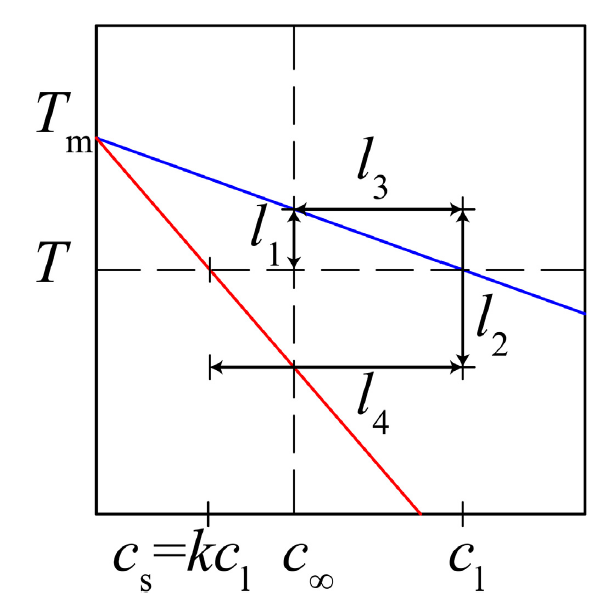
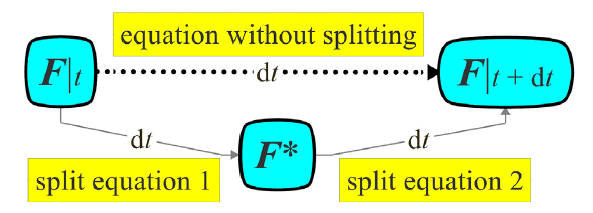

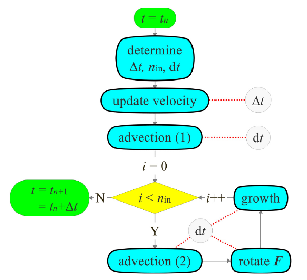
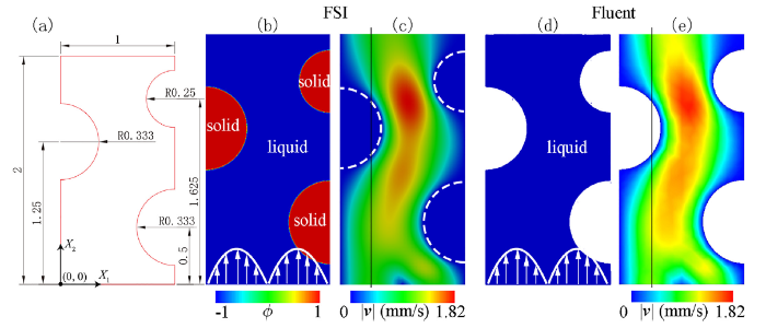
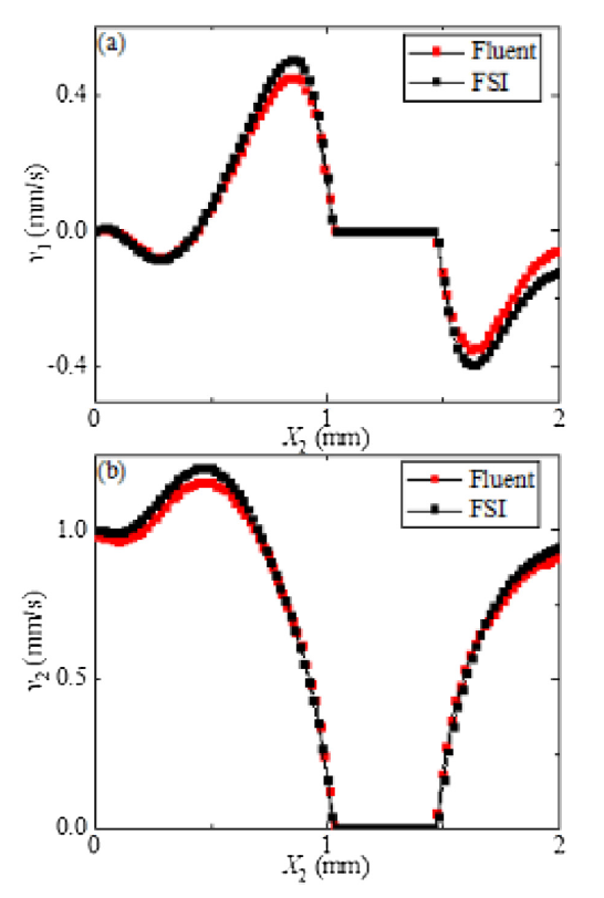
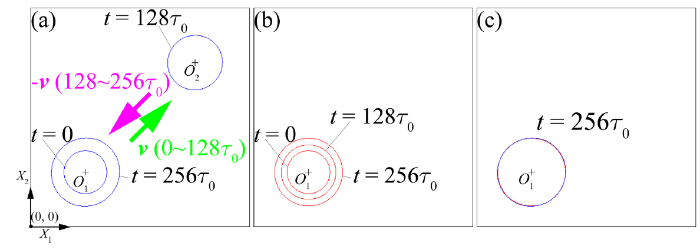
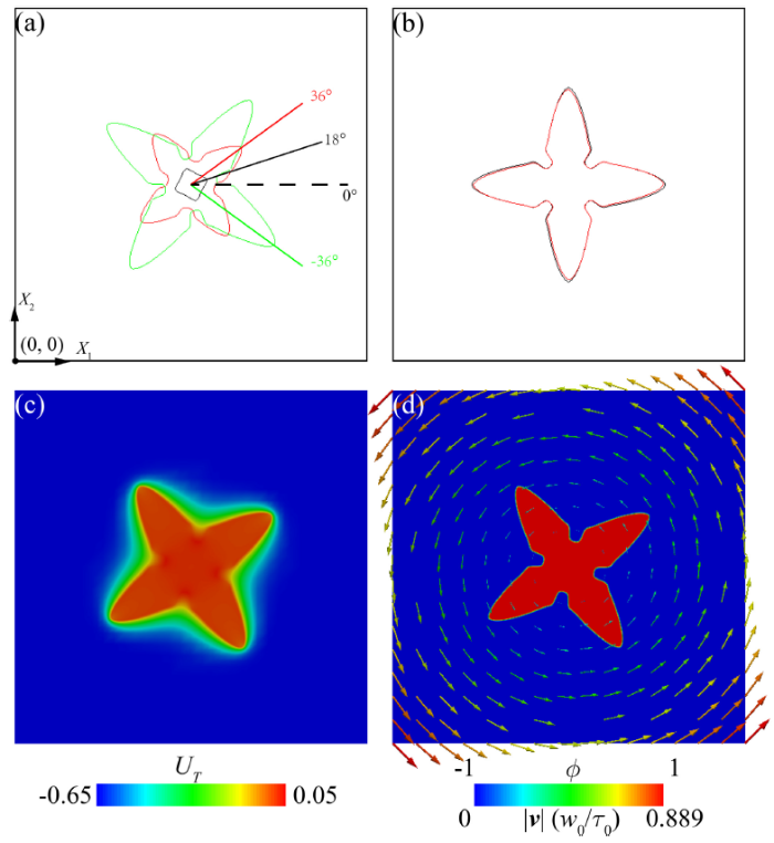
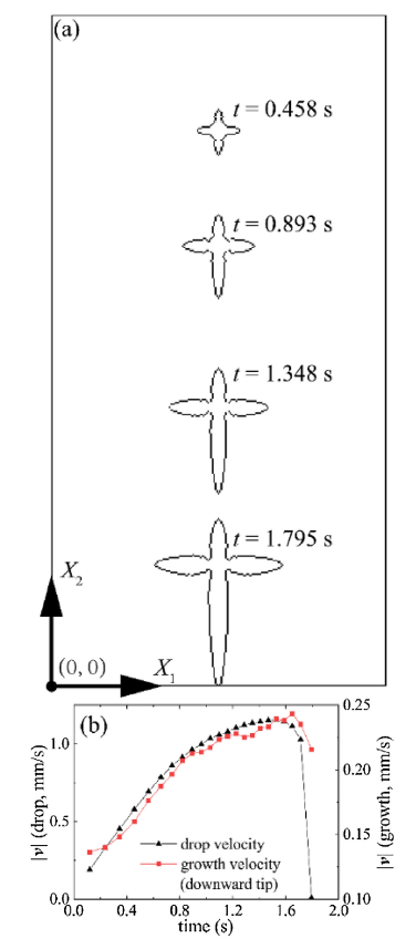
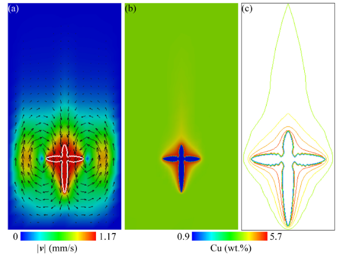

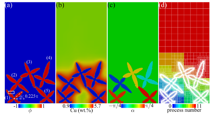
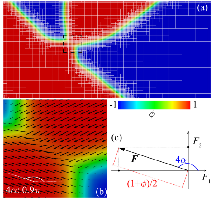
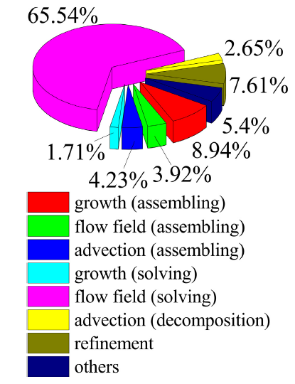

 WeChat