Search for articles:
Qing Liu, He junLi , Yulei Zhang, Zhigang Zhao
Corresponding authors:
Received: 2018-07-26
Accepted: 2018-10-23
Online: 2019-05-10
Copyright: 2019 Editorial board of Journal of Materials Science & Technology Copyright reserved, Editorial board of Journal of Materials Science & Technology
More
Abstract
Multi-layer connected self-organizing feature maps (SOFMs) and the associated learning procedure were proposed to achieve efficient recognition and clustering of messily grown nanowire morphologies. The network is made up by several paratactic 2-D SOFMs with inter-layer connections. By means of Monte Carlo simulations, virtual morphologies were generated to be the training samples. With the unsupervised inner-layer and inter-layer learning, the neural network can cluster different morphologies of messily grown nanowires and build connections between the morphological microstructure and geometrical features of nanowires within. Then, the as-proposed networks were applied on recognitions and quantitative estimations of the experimental morphologies. Results show that the as-trained SOFMs are able to cluster the morphologies and recognize the average length and quantity of the messily grown nanowires within. The inter-layer connections between winning neurons on each competitive layer have significant influence on the relations between the microstructure of the morphology and physical parameters of the nanowires within.
Keywords:
Nanowires (NWs) are one-dimensional nanomaterials that have applications in many fields including advanced functional sensors, electronic devices and ideal reinforcements in composites [1], [2], [3], [4], [5], [6], [7], [8]. The properties of nanowires are usually achieved by their unique shapes and morphologies. Nanowire morphologies can be generally divided into two categories - aligned nanowires or messily grown nanowires [9]. Morphologies formed by messily grown nanowires usually consist of a large quantity of nanowires with different lengths and random growing directions. The messily grown nanowires are usually bending, crossing or overlapping with each other, forming the complex, disordered but uniform network-structures [9,10]. The network formed by messily grown nanowires are ideal candidates for functional sensors or reinforcements of structural composites [1,2,[6], [7], [8], [9],11].
For design and synthesis of nanowire reinforcements, efficient recognition, classification and estimation of the microstructure, quantity and length of messily grown nanowires are necessary. However, such information is difficult to obtain. On one hand, the complex microstructure and large quantity make it difficult to obtain the details of the density, quantity and length of messily grown nanowires. On the other hand, though the microstructure of the morphology is determined by quantity growth and elongation of nanowires within, relations between the microstructure of the morphology and the growth of nanowires are difficult to identify. Fortunately, neural networks have the ability to approximate an arbitrary function by learning from the observed data [12]. Thus, it is desirable if we can use neural networks to recognize, classify and estimate the microstructure, quantity and length of the messily grown nanowires by means of teaching it to “learn” the relations between microstructural factors and physical parameters of messily grown nanowires.
Artificial neural networks (ANNs) are a family of information processing systems simulating both functionality and structure of biological neural networks. Similarly to the learning process of human brain, the learning procedures in ANN contains both unsupervised and the supervised learning [13], [14], [15]. Since the unsupervised learning is self-organized and automatically accomplished, it will be desirable if the neural network can be trained by unsupervised learning procedures. One kind of ANNs called self-organizing feature maps (SOFMs) which is designed for unsupervised learning may be suitable.
SOFM was first proposed by Kohonen in 1980s [14,16,17]. In his view, a neural network would be divided into several regions according to the input patterns. Neurons in each region show different reactions to the input patterns. The process of neuron rearrangements is automatically accomplished. Based on this idea, the concept of self-organizing map was then proposed. A SOFM system is usually made up by an input layer and a 2-D competitive layer [16]. The input layer receives and transmits the input signals to the competitive layer. On the competitive layer which is made up of 2-D neuron arrays, self-organizing competition is carried out. The winner of the competition will have the right to make response to the input modes while others are restrained [16,18]. SOFM is a neural network designed as a method for clustering and has been employed to solve different kinds of data clustering tasks [15,19,20]. SOFM can generate a feature map formed by similar groups of the input modes through unsupervised learning. This is usually accomplished by similarity analysis between neurons on the competitive layer and the input modes. Each neuron on the competitive layer contains a weight vector which has the same dimension as the input space [16]. The weight vectors are updated through the self-organizing learning process, resulting in neurons rearrangements according to modes in the input space [18].
The purpose of this work is to design a new structure of SOFMs and the associated algorithm for efficient recognition of morphologies formed by messily grown nanowires. Firstly, the structure was created by connecting several layers together, each of which is a classical (single-layer) SOFM consisting of Kohonen units. The overall structure is in the form of several paratactic connected competitive layers. Each of the layers is able to build connections with the neighboring layers according to the mapping relations between the training samples input on each layer. Secondly, virtual training samples were generated by a large amount of Monte Carlo simulations. Then, the network was trained by the virtual samples to build connections between structural factors of the morphology and physical parameters of the nanowires within. Afterwards, the as-trained SOFMs were applied on the task of clustering and recognizing the microstructure, quantity and length of the messily grown nanowires synthesized by experiments.
2.1.1. Topology structure
In this section, the double-layer connected SOFMs are used as the simplified model since the multilayer connected ones can be generalized from the double-layer situation. The structure of double-layer connected SOFMs is schematically illustrated in Fig. 1(a). Every single layer is a 2-D SOFM competitive layer named as layer N1 and N2 respectively. The weights of neurons on layer N1 and N2 are noted as W and V respectively. Then, neurons on the two layers have potential inter-layer connections with the weights noted as 12$W_{N2}^{N1}$, where the superscript and the subscript are corresponding to the neurons on N1 and N2 respectively.
Fig. 1. Topology structure of the connected double-layer SOFMs [(a)] and numbering rules of neurons on each layer [(b)].
To make a clear description of the neuron states, it is necessary to give sequence numbers to each neuron. Assuming that layer N1 and N2 are formed by neuron arrays with size of n × n, a 2-D coordinate system can be built up with one of the vertex neuron as the base point, as shown in Fig. 1(b). The sequence numbers of neurons are counted starting with the base point and increasing from the left to the right side of x axial and from the bottom to the top of y axial. For layer N1 and N2, the neuron numbers are noted as i = 1, 2, 3, …, n2 and j = 1, 2, 3, …, n2 respectively. Thus, the weights of neurons on each layer can be expressed as W=( W1,W2,...,Wn2) and V=( V1,V2,...,Vn2). Similarly, the weights of the inter-layer connections are written as 12$W_{N2}^{N1}$=12$W_{•}^{1}$,12$ W_{•}^{2}$•,...,12 $W_{•}^{n^{2}}$ or 12$W_{N2}^{N1}$=12$W_{1}^{•}$1•,12$W_{2}^{•}$,...,12$ W_{ n^{2}}^{ •}$, where 12$W_{•}^{ i }$ is the inter-layer weights between neuron i on N1 and all neurons on N2, 12$W_{j}^{•}$the inter-layer weights between neuron j on N2 and all neurons on N1.
2.1.2. Training method
The new structure of SOFMs is trained by the self-organized learning algorithm. Let X and Y be a group of training samples with sample size k and functional relation expressed as Y = f (X). In order to achieve clustering analysis and to identify the mapping relations of X and Y, it is necessary to form the cluster feature maps on each SOFM layer by means of inner-layer learning and build up the connections among different layers via inter-layer learning.
According to the topology structure of the networks, the training samples are input into each SOFM layer respectively. For SOFM layers, Kohonen algorithm is used. Kohonen algorithm is developed from the so-called ‘Winner-Take-All (WTA)' competition in which similarity measurements are carried out between the input mode and the neurons. The winner exhibiting the highest similarity with the input mode is active while others are restrained and keep silence [21,22].
Kohonen algorithm is carried out as follows: firstly, the input modes and the weight vectors need to be normalized as

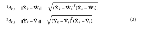
Secondly, similarity analysis between the input modes and the weights of neurons are carried out on each competitive layer. Herein, the similarity is measured by calculating Euclidean distances between the neuron weights and the input training samples, yielding
In Kohonen algorithm, the weights updating rules are different from WTA. The response of neurons varies with the distance away from the winning neuron. An area called the winning neighbor domain is introduced to identify the neighboring neurons of the winner. The winning neighbor domain refers to the region within a topology radius dN from the central winning neuron. All neurons within the winning neighbor domain have the chance to update their weights according to their distance from the central winning neuron while the ones outside the zone are restrained and cannot update their weights. Thus, the learning rate of Kohonen algorithm can be expressed as the function of winning neighbor domain and training times:
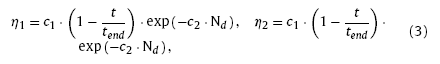
where c1 and c2 are model coefficients, tend the total train time, dNi,i* the topology distance between neuron i and winning neuron i* on N1, dNj,j* the topology distance between neuron j and the winning neuron j* on N2. For convergence of the algorithm, the size of the winning neighbor domain is also narrowing down gradually with the increasing training times, yielding
$N_{d}=c_{3}·n·(1-\frac{t}{t_{end}})$, (4)
where c3 is size coefficient and n the number of neurons along the edge of the competitive layer. Usually, c3 is varying from 0 to 1 to ensure the size of the winning neighbor domain not exceeding the size of competitive layer. Finally, with Eqs. (3)and (4), the weights updating equations of neurons within the winning neighbor domain are given as
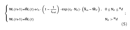
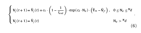
Besides the inner-layer learning for clustering of the training samples, it is also necessary for the networks to learn the mapping relation\s between X and Y during training. In order to build up the inter-layer connections, the response function for each layer is necessary to be introduced. Response functions need to satisfy conditions as follows: 1. the winning neuron has the strongest response; 2. neurons outside the winning neighbor domain have zero responses; 3. Responses of neurons inside the winning neighbor domain are narrowed down with the increasing distance from the winning neuron. According to the conditions mentioned above, the response functions of layer N1 and N2 can be given as
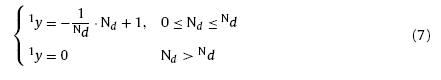
and
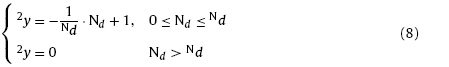
where 1y and 2y are response functions of layer N1 and N2 respectively. The response functions can give information about the distribution of the winning neurons and the ones located in the winning neighbor domain on each competitive layer. With Eqs. (7) and (8), the position and strength of the inter-layer connections can be identified.
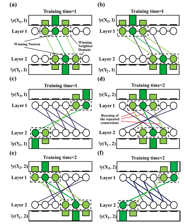
For the purpose of learning the mapping relation between sample Xˆm and Yˆm, it is necessary to build up the inter-layer connections between the winning neurons which are sensitive to Xˆm and Yˆm respectively and boost the repeating connections during training. Information of the mapping relation can be finally transformed into the inter-layer connecting patterns. The inter-layer learning should comply with rules as follows: 1. Neurons with zero response cannot connect with each other; 2. Neurons with similar response tend to have strong connections; 3. the higher response a neuron shows, the stronger connections it has; 4. repeating connections are boosted with the increasing training times. The process of the inter-layer learning is shown in Fig. 2. Thus, the weights updating equation of inter-layer connections can be given as
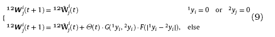
Fig. 2. Schematic of inter-layer learning procedure. (a)-(c) Building inter-layer connections between winning neurons and the neighbored ones representing the training samples with mapping relations; (d)-(f) boosting of the repeated connections.
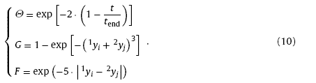
where Θ(t), G(1yi,2yi) and F(|1yi-2yi |) are learning functions. Function Θt is the increasing function of training times, suggesting the continuous boosting of the repeating connections; G(yi,yi) is the increasing function of the neuron responses 1yi and 2yj, suggesting the strong connections between highly responding neurons; F(|1yi-2yi |) scales inversely with |1yi-2yi |, indicating that neurons with similar response tend to have strong connections. There could be many options for the selection of learning functions complying with the above mentioned rules. Herein, the learning functions are selected as
2.1.3. Response to new inputs
After the training process, the neural network could classify and make predictions for the newly input patterns. Since the clustering and mapping information of the training samples have already been transformed into the patterns of inner-layer and inter-layer connections, it is important to compare the newly input patterns with neurons of the as-trained networks. Considering the double-layer situation, let Xp be the new mode put into layer N1 (noted as the input layer during response process), the stress reactions of neurons on the input layer can be calculated by

where c4 is constant. Eq. (11) indicates that neuron exhibiting the highest similarity with Xp shows the strongest stress reaction. Then, the excitatory neuron noted as iS will trigger the reactions of winning neurons on the same layer. The stress reactions of the triggered winning neurons on input layer is determined by

In Eq. (12), coefficient c5 is calculated by
$c_{5}=\frac{ln(o_{min})}{max(\parallel \hat{W}_{i_{s}}-\hat{W}_{i*}\parallel)}$ (13)
where omin is the expected min stress reaction of the triggered winning neurons on input layer. Afterwards, neurons on layer N2 (noted as the stress reacting layer during response process) will be stimulated by the triggered winning neurons on input layer because of the inter-layer connections. Thus, the output of the stress reacting layer can be calculated by
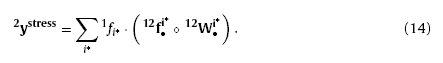
where “∘” is the multiplications of the corresponding elements of two vectors; f1i* and 12f•i* are the flitters which can reinforce the strong factors and restrain the weakness ones to make the results more significant. Herein, expressions of the flitters are given as
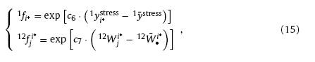
where c6 and c7 are positive coefficients, 1y¯stress the average stress reaction of the triggered winning neurons on input layer, 12W¯•i* the average of inter-layer connections of winning neuron i*. Eq. (15) suggests that the flitters are more than 1 when the neural response or inter-layer connections are higher than the average levels, making the results reinforced; on the contrary, the flitters become less than 1 as the corresponding factors are lower than the average levels, resulting in the restrained results. Finally, the prediction of Xp can be obtained through the outputs of winning neurons on the stress reacting layer. The probability of training sample Ym being the prediction of Xp can be calculated by
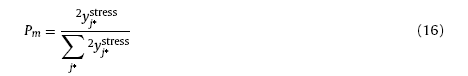
where 2yj*stress is the output of winning neuron j* on stress reaction layer. With Eq. (16), the network prediction for Xp is the weighted average of training samples yielding
$Y_{p}=P^{T}·Y=\sum_{m}P_{m}·Y_{m}$ (17)
As is widely known, the functioning of ANN depends on the training samples. Thus, large amount of messily grown nanowire morphologies must be prepared as the training samples to ‘teach' the neural network to cluster and recognize the morphological features. However, it is difficult to obtain large amount of such morphologies with different nanowire quantities and lengths by experiments. Herein, we propose an algorithm to solve this problem by replacing the experimental training samples with the virtual ones generated by Monte Carlo simulations. Our simulation is carried out in a squared zone with area of L×L. Firstly, growing points with quantity of Nsim are randomly distributed in the simulated area. Then, virtual nanowires with length lsim and radius rsim are grown from these points and forming the virtual morphology.
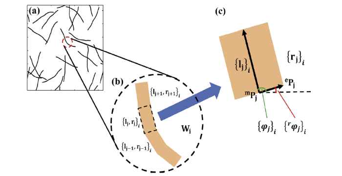
Let Msim=(NW1,NW2,...,NWi,...,NWNsim )be the virtual morphology including nanowires noted as NW1, NW2,…, NWNsim. Each virtual nanowire is formed by a series of one-by-one connected line sections with length of Δl and different directions, as shown in Fig. 3. Each line section is described by growth vector and radius vector noted as {lj}i and {rj}i respectively. The vectors can be expressed as [9]
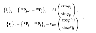
Fig. 3. Model of the virtual training samples. (a) Generated virtual morphology of messily grown nanowires; (b) and (c) structure of the virtual nanowire and each line section.
where mPj = (mxj, myj)T and ePj = (exj, eyj)T are the starting and terminal point of the radius vector respectively, Δl and rsim (also the radius of virtual nanowire) the length and width of the line section, φij and rφij the direction angles of the growth vector and radius vector respectively. Thus, the growth of virtual nanowire can be described by the following iteration [9]:
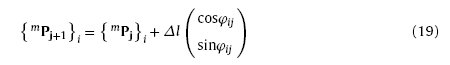
with
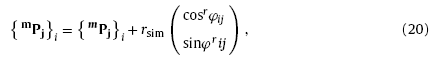
where rφij=φij-π2. In order to achieve the varying growth direction, φij is determined by the random sampling process from a statistical population. Herein, φij was assigned from a uniform distribution yielding φij∼Uφij-1-Δφ,φij-1+Δφ [9]. Δφ controls the curving of the virtual nanowire [9], it is treated as a free parameter in the Monte Carlo simulation. According to the proposed simulation method, virtual training samples with different nanowire quantities, lengths, radii and Δφ can be generated.
After obtaining the virtual morphologies, it is still needed to describe their microstructures with a group of parameters which can be easily recognized by neural networks. To achieve this, the virtual morphology is firstly adjusted to the squared size and meshed by a series of tiny grids with size of ε0 × ε0. Then, the numbers of grids covered by nanowires is counted line by line along x and y direction respectively. According to this model, the density or fraction of virtual nanowires in the morphology can be described by calculating the ratio of the area covered by nanowires and the total area yielding
$\rho_{A}=\frac{N_{c}(\varepsilon_{0})·\varepsilon_{0}^{2}}{L^{2}}$, (21)
where ρA is called the actual area ratio, Nc(ε0) the total number of grids covered by virtual nanowires. Besides, information about the distribution of virtual nanowires within the 2-D morphology can be given by counting the numbers of covered grids in each column along x and y directions respectively. Thus, we have
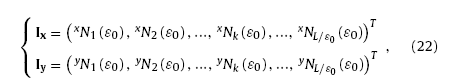
where Ix and Iy are image vectors, xNk (ε0) and yNk (ε0) the numbers of covered grids in column k along x or y direction, L/ε0 the total column number of the virtual morphology [9]. According to Eq. (22), the fraction of the covered grids (also called covered fraction or CF) in column k can be calculated as
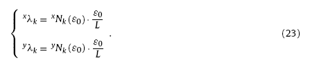
With Eq. (23), the image vectors can be further written as
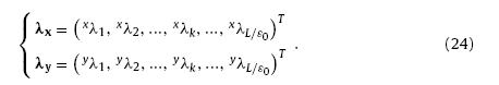
According to Eq. (24), the histograms of λx and λy can be obtained by statistical method. The CF histograms noted as H(λx) and H(λy) give structural information of the virtual morphology [9].
Since the simulations are carried out in the squared area with size of L×L, the virtual morphologies may in different sizes from the experimental ones. Thus, it is necessary to develop the size transformation rules which can achieve conversions of nanowire lengths and growth directions between experimental and simulated morphologies. The coordinate transformation equations for nanowire length and growth directions have been proposed in our previous work [9]:
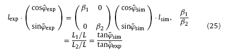
where β1 and β2 are scale factors, L1 and L2 the length and width of the experimental morphology, φ¯exp and φ¯sim the average growth direction of experimental and virtual nanowires.
In summary, microstructure of the simulated morphologies can be quantitative described by parameters including actual area ratio (ρA), image vectors (Ix & Iy) and CF histograms [H(λx) & H(λy)] together with nanowire quantity (Nsim), length (lsim), radius (rsim) and growth direction change (Δφ).
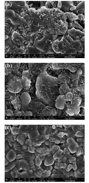
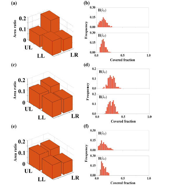
In this section, the as-proposed algorithm was applied on clustering and pattern recognition of messily grown Si nanowires reported in our previous work [9]. The SEM images of the experimental morphologies are shown in Fig. 4. The morphologies in Fig. 4(a)-(c) are noted as M1 (grown for 2 h at 950 °C), M2 (grown for 2 h at 1000 °C) and M3 (grown for 0.5 h at 1100 °C) respectively. Each of the morphologies is divided into the upper left side (UL), upper right side (UR), lower left side (LL) and lower right side (LR) respectively [9]. The average nanowire diameter, length, growth direction and change of the growth direction of M1-M3 are shown in Table 1. Area ratios and CF histograms of M1-M3 were calculated and shown in Fig. 5. It can be seen that the area ratios of M2 and M3 are uniform distributed except M1 in which the area ratio of M1-UR is obviously larger than other parts, suggesting the denser nanowire networks on the upper right side of M1. It also can be seen in Fig. 5 that M1 and M3 show similar actual area ratios though the average nanowire length is different, indicating that the actual area ratio is not influenced by single nanowire parameter but holistically related to nanowire quantity, length and radius [9].
Fig. 4. SEM images of messily grown Si nanowire morphologies [
Fig. 5. Area ratios and CF histograms of experimental morphologies M1 [(a) and (b)], M2 [(c) and (d)] and M3 [(e) and (f)].
Table 1 Average converted radii, nanowire length, direction angles and growth direction change of morphology M1-M3 [
| ρA | 2rexp (nm) | rconv | lexp (μm) | φ¯(deg) | Δφ(deg) | |
|---|---|---|---|---|---|---|
| M1 | 0.133 | 26.89 | 0.098 | 0.56 | 81.83 | 9.27 |
| M2 | 0.273 | 27.74 | 0.085 | 1.80 | 93.29 | 7.85 |
| M3 | 0.128 | 29.14 | 0.050 | 1.46 | 96.06 | 5.20 |
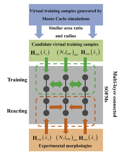
The pattern recognition of messily grown nanowires mainly includes two steps (see in Fig. 6). The first step is to find the candidate set which is formed by virtual training samples with similar area ratio and converted radius to the experimental morphology. Herein, the “converted radius” is the radii of experimental nanowires under simulation coordinate system. The converted radius is obtained by two steps. Firstly, change the experimental morphologies into squared size and measure pixel numbers of the “width” of nanowires. Then, the converted radius of experimental nanowires can be calculated by
$r_{conv}=\frac{N_{p}(2r)}{N_{p,total}}·\frac{L}{2}$ (26)
Fig. 6. Schematic of morphology recognition using the as-proposed SOFMs.
where Np(2r) is the pixel numbers of nanowire's width, Np,total the pixel numbers of morphology's edge. The converted radii make it possible to compare the radii of experimental nanowires with the virtual ones.
After the determination of candidate set, the training samples are obtained by organizing the nanowire quantity, nanowire length, CF histograms along x and y directions of each candidate (see in Fig. 6). Thus, the training samples can be expressed as
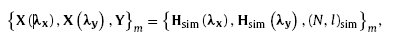
where the mapping relations of Xmλx→Ym and Xmλy→Ym are satisfied. The nanowire quantity and length of the candidate training samples for M1∼ M3 are shown in Table 2.
Table 2 Candidate sets including virtual training samples with similar area ratios to the experimental morphologies.
| Candidate set with nanowire quantity and length (Nsim, lsim) | |||||||
|---|---|---|---|---|---|---|---|
| M1 | UL | rsim = 0.1 | (50,5) | (70,3.5) | (100,2.5) | - | (200,1) |
| UR | (50,10) | (70,8) | (100,5) | (150,3) | (200,2.5) | ||
| LL | (50,6) | (70,4.5) | (100,3) | (150,2) | (200,1.5) | ||
| LR | (50,5) | (70,3.5) | (100,2.5) | - | (200,1) | ||
| M2 | UL | rsim = 0.05 | - | (70,17) | (100,10) | (150,6) | (200,4.5) |
| rsim = 0.1 | - | (70,12) | (100,8) | (150,4.5) | (200,3.5) | ||
| UR | rsim = 0.05 | - | (70,25) | (100,13) | (150,8) | (200,6) | |
| rsim = 0.1 | - | (70,17) | (100,10) | (150,6) | (200,4) | ||
| LL | rsim = 0.05 | - | (70,17) | (100,10) | (150,6) | (200,4.5) | |
| rsim = 0.1 | - | (70,12) | (100,8) | (150,4.5) | (200,3.5) | ||
| LR | rsim = 0.05 | - | (70,15) | (100,9) | (150,6) | (200,4) | |
| rsim = 0.1 | - | (70,10) | (100,7) | (150,4) | (200,3) | ||
| M3 | UL | rsim = 0.05 | (50,10) | (70,6.5) | (100,4) | (150,2.5) | (200,2) |
| UR | (50,10) | (70,7) | (100,4) | (150,3) | (200,2) | ||
| LL | (50,8) | (70,5.5) | (100,4) | (150,2.5) | - | ||
| LR | (50,7) | (70,5) | (100,3) | (150,2) | - | ||
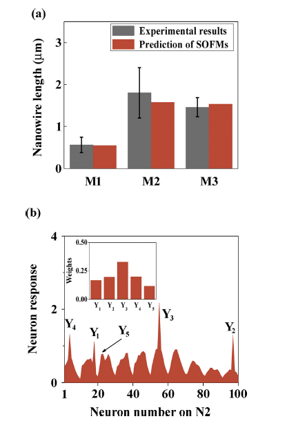
According to the candidate set of virtual training samples, three-layer connected SOFMs with 10×10 neuron array are trained for 300 times. During training, Xm(λx), Ym and Xm(λy) were respectively input into each competitive layer of the networks (see in Fig. 6) to form the inter-layer connections. After the training process, the as-trained network was then used to classifying the microstructure and recognizing the nanowire length and quantity of experimental morphologies. The predictions of nanowire length of M1-M3 are shown in Fig. 7(a). It can be seen that the as-trained network is able to give reasonable length predictions to experimental messily grown nanowires based on the virtual training samples, the estimated nanowire quantities are shown in Table 3.
Fig. 7. Nanowire length predictions and neuron responses of the as-trained double-layer SOFMs. (a) Nanowire length of the experimental morphologies predicted by the as-trained SOFMs; (b) neural responses to input H(λx) of M3-UL.
Table 3 Estimated nanowire quantity and length of experimental morphologies.
| N˜exp | l˜exp (μm) | |
|---|---|---|
| MM1 | 488 | 0.55 |
| MM2 | 478 | 1.58 |
| MM3 | 465 | 1.53 |
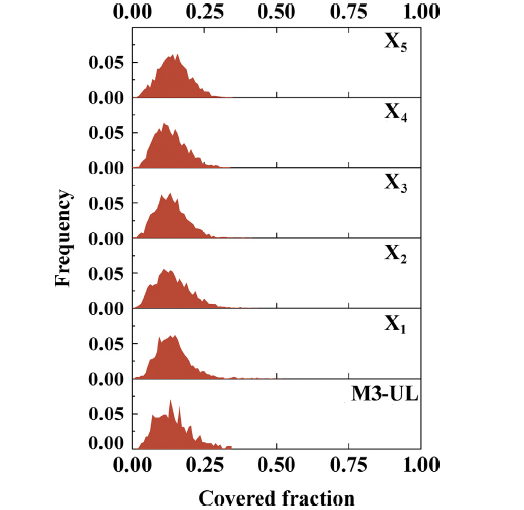
For analyzing the neuron states of the as-trained networks, the training process of the upper left side of M3 (M3-UL) is mainly discussed in this section. The mapped candidate training samples of M3-UL are written as

The detail information of these samples is shown in Fig. 8 and Table 2.
Fig. 8. H(λx) of M3-UL and the virtual training samples with similar ρA and rsim to M3-UL.
The stress reactions of neurons in response to the input Hexpλx are shown in Fig. 7 (b). It is found that winning neuron representing sample Y3 show the active response, suggesting that the input morphology is most probably treated as the same cluster with sample Y3 in which the nanowire quantity and length are of (100,4).
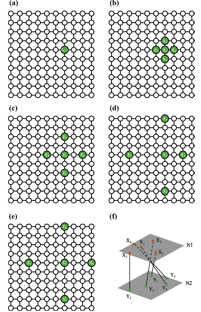
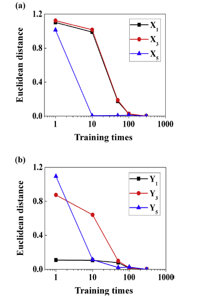
The evolution of the winning neuron locations on layer N1 is shown in Fig. 9. From Fig. 9 we can see that the winning neurons are gathered at the single position as the training begins. With the increase of training times, locations of winning neurons become quickly separated and gradually stabilized, suggesting that the training samples have been clustered at the early training stage and been adjusted and consolidated till the end of training. The evolution of Euclidean distance between the final winning neurons and the represented training samples is shown in Fig. 10. It can be seen that the Euclidean distance between the final winning neuron and the represented training sample is rapidly disappeared during training process. The results in Fig. 10 show that the clustering information of training samples has been mapped into the locations of the winning neurons on competitive layers. Furthermore, the Euclidean distance experiences a drastic decrease only in the early training stage within 100 times. Then, the Euclidean distance tends to keep stable during the subsequent training. This indicates that the clustering maps are formed by the network during early training stage and then are boosted continuous in the later training stage.
Fig. 9. Evolution of winning neuron locations with training times on layer N1. The inputs are candidate virtual training samples for M3-UL. Winning neuron locations with (a) 1 training time, (b) 10 training times, (c) 100 training times, (d) 200 training times, (e) 300 training times. (f) Final location and inter-layer connection of winning neurons.
Fig. 10. Evolution of Euclidean distance between winning neurons and the corresponding training samples. The inputs are candidate virtual training samples for M3-UL. (a) Distance evolution of X1, X3 and X5 on layer N1; (b) distance evolution of Y1, Y3 and Y5 on layer N2.
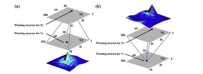
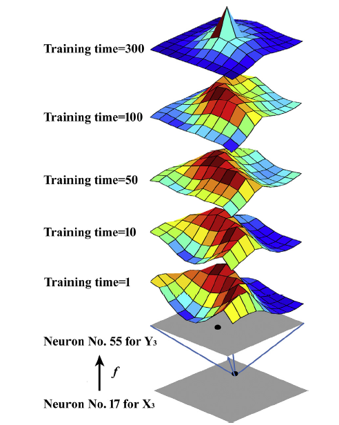
The inter-layer connections between the winning neurons representing a couple of mapped training samples are shown in Fig. 11. Max weights between the coupled winning neurons are found, suggesting that the strong inter-layer connection between the two neurons has been formed. Evolution of the inter-layer connections of winning neurons is shown in Fig. 12. It can be seen that winning neuron No.17 on N1 is not only strongly connected with the target winning neuron No.55 on N2 but also with many other neurons. As the training moves on, connection with the target winning neuron is then boosted continuously. At final stage of training, only the connection with target winning neuron (Neuron No.55) becomes the strongest. The results in Fig. 12 indicate that the as-proposed networks have the ability to learn the mapping relations between training samples by inter-layer learning algorithm.
Fig. 11. Inter-layer weights of winning neurons representing Hλx and Nsim,lsim of one virtual training sample {X3(λx),Y3}. Numbers on the edges of N1 and N2 represent the sequence number of the neurons. (a) Inter-layer connections of winning neuron No.17 on layer N1; (b) inter-layer connections of winning neuron No.55 on layer N2.
Fig. 12. Evolution of inter-layer weight of winning neuron No. 55 on layer N2 representing Y3 X3.
Microstructures, average quantity and length of messily grown nanowires are classified and recognized by a novel structure of connected multilayer SOFMs. The morphological features and average nanowire quantity and length can be clustered and predicted by the as-proposed network trained through virtual training samples generated from Monte Carlo simulations. The virtual training samples can replace the “real” ones synthesized by experiments to make the training faster and more efficient.
During the training process, the inter-layer connections between winning neurons on each competitive layer representing the mapped training samples are formed and boosted. The relations between the mapped training samples are successfully transformed into the inter-layer connecting patterns. The results of similarity probability also show that experimental morphologies are classified by the SOFMs according to the clustering map of virtual training samples after self-organizing learning.
This work has been supported by the National Natural Science Foundation of China under Grant Nos. 51727804 and 51672223, and supported by the “111” project under grant No. B08040.
The authors have declared that no competing interests exist.

 WeChat
/
| 〈 |
|
〉 |
