During a hypothetical severe accident of light water reactors, the reactor pressure vessel (RPV) could fail due to its creep under the influence of high-temperature corium. Hence, modelling of creep behavior of the RPV is paramount to reactor safety analysis since it predicts the transition point of accident progression from in-vessel to ex-vessel phase. In the present study we proposed a new creep model for the classical French RPV steel 16MND5, which is adapted from the “theta-projection model” and contains all three stages of a creep process. Creep curves are expressed as a function of time with five model parameters θi(i=1-4 and m). A model parameter dataset was constructed by fitting experimental creep curves into this function. To correlate the creep curves for different temperatures and stress loads, we directly interpolate the model’s parameters θi(i=1-4 and m) from this dataset, in contrast to the conventional “theta-projection model” which employs an extra single correlation for each θi(i=1-4 and m), to better accommodate all experimental curves over the wide ranges of temperature and stress loads. We also put a constraint on the trend of the creep strain that it would monotonically increase with temperature and stress load. A good agreement was achieved between each experimental creep curve and corresponding model’s prediction. The widely used time-hardening and strain-hardening models were performing reasonably well in the new method.
Peng Yu, Weimin Ma. A modified theta projection model for creep behavior of RPV steel 16MND5. Journal of Materials Science & Technology[J], 2020, 47(0): 231-242 DOI:10.1016/j.jmst.2020.02.016
1. Introduction
Creep is an irreversible time-dependent inelastic deformation process which happens as long as there is a stress. The molecular mechanism of creep can be generally classified as diffusion and dislocation, the former of which normally occurs due to the presence of vacancies within the crystal lattice (or the grain) while the latter occurs if there is a slip by the passage of crystal dislocations [1]. There are two types of diffusion creep [2], called Coble creep (favored at lower temperatures) if the diffusion paths are predominantly through the grain boundaries, and Nabarro-Herring creep (favored at higher temperatures) if through the grains themselves. This mechanism of creep tends to dominate at high stresses and relatively low temperatures. Dislocations can move by gliding in a slip plane, a process requiring little thermal activation. However, the rate-determining step for their motion is often a climb process, which requires diffusion and is thus time-dependent and favored by higher temperatures. The creep behavior is highly dependent on temperature and stress: creep can be negligibly small under low temperature and stress; it occurs faster at higher temperature and stress. Generally, it is expected that creep rate would have an exponential dependence on temperature for steady-state creep as shown in Eq. (1) and a power dependence on stress as expressed in Eq. (2):
where $\dot{\varepsilon }$ is the creep strain rate, Q is the activation energy associated with the rate, R is the universal gas constant (= 8.31 J/mol/K), T is the temperature in K, and σ is the stress.
A creep curve describes the creep strain development with time under constant stress and temperature as shown in Fig. 1. Typical creep curves can be characterized by three stages: primary stage where the creep strain rate decreases with time, secondary stage where the creep strain rate almost keeps constant and tertiary stage where the creep strain rate drastically increases with time.
Fig. 1.
Creep curve under constant temperature and stress.
In the engineering modelling of kinematics for deformation and motion, the creep effect is considered by introducing extra terms into the conservation equations. To close the equation sets, a creep model (a constitutive equation describing the creep strain or creep strain rate as functions of stress, temperature, time and creep strain.) is required. There are many creep models available for creep simulations, ranging from simple-phenomenological to complex-constitutive ones. Commonly used models include the typical time hardening and strain hardening models for primary stage of creep; Norton’ Law [3] and Exponential form for the secondary stage of creep; Norton-Bailey, RCC-MR [4] and Bartsch [5] for both the primary and secondary stages; Theta Projection [1], Rabotnov-Kachanov [6], Baker-Cane [7] and Dyson-McLean [8] for all three stages.
The commercial software ANSYS [9] and ABAQUS [10] have default standard creep models that only include the primary and/or the secondary stage(s). The two codes offer the interfaces to implement user-defined creep laws through either ANSYS User Program Functions or ABAQUSs user subroutines. One reason why the tertiary stage is not modeled by default might be that for most industrial applications the failure analysis is beyond interest, and therefore the built-in creep laws in the commercial software is supposed to be sufficient [11]. The extra user-defined creep law should be implemented when a user is interested in the tertiary creep stage and/or wants more accurate creep modelling.
The steel 16MND5 is a typical material widely used to construct the reactor pressure vessel (RPV). 16MND5 is a low-alloyed ferritic steel whose chemical composition is given in Table 1 [12,13]. It has undergone several heat treatments during its elaboration: two austenizations followed by water quench, a tempering and a stress-relief treatment which then lead to a ‘tempered bainite’ structure. Since the RPV also serves as the second physical barrier to contain the core material and prevent radioactivity release under operations and accidents, its integrity is of great importance to nuclear power safety. A severe accident with core meltdown may threaten the RPV integrity, since the relocated reactor core melt (corium) in the RPV lower head will exert thermal and mechanical loads on the vessel wall, which may ultimately lead to vessel failure due to creep under the high temperature and significant stress. The “vessel failure due to creep” means that the lower head wall does not only go through the primary and secondary stages, but also reaches the tertiary stage of creep. Hence, accurate modelling of creep in three stages is important to RPV integrity assessment during a hypothetical severe accident.
Table 1
Table 1Chemical composition of 16MND5 steel (weight-%).
For the creep behavior of the 16MND5 steel, the REVISA Experiment [14] at CEA performed the tensile and creep tests using 16MND5 specimens at a wide range of temperature from 600 °C to 1300 °C. Four tests with different stress loads were carried out for each temperature. It provided the most important experimental data of the creep behavior of 16MND5. Several treatments have been explored to correlate the experimental data into numerical analysis of structural integrity. Iknoen [15] fitted the data of the REVISA experiment into a three-stage creep model: three creep stages are distinguished by separate correlations, and creep at each stage is described by a time-hardening model with different temperature-dependent coefficients. Altstadt and Moessner [16] transferred the experimental curves to a discretized database: under each given temperature T and stress σ, the creep curve was discretized into finite point pairs (ε, $\dot{\varepsilon }$) indicating under such thermal and mechanical loads the creep strain rate $\dot{\varepsilon }$ is subjected to creep strain ε. The creep strain rate for any other case can be interpolated over known temperature, stress, and strain from the database. Due to the limited information, we do not know the performance of such approach. Willschutz et al. [17] adopted this database idea and used in their creep failure simulation. A different treatment [18] was later proposed to predict the creep strain acceleration in the tertiary stage. A correction factor 1/(1-D) was introduced to the creep strain increment, where D is a damage factor (0<D<1). (The usage of such damage variables was initially proposed by Kachanov [19] and Rabotnov [20]. A related review can also be found in [21].) In this research, D was defined by both creep and plasticity information. As damage parameter grows close to 1, the creep strain rate would be enlarged more significantly as is multiplied by this factor 1/(1-D). The comparison [22] between model predictions and experimental data shows that, the model can predict three-stage creep behavior and generally agrees with the experimental data. However, large discrepancies exist in a good number of creep curves: regarding the time reaching the same strain, 8 out of 32 curves show a discrepancy of ∼100% between prediction and experiment; 5 more curves show a discrepancy of ∼25%. Moreover, it is noted this damage factor is dependent on plastic performance, and therefore a change in plastic model might numerically have influence on the creep prediction.
As the creep model plays a pivotal role in modelling vessel failure during a severe accident, there is a clear need to improve its fidelity for a more credible RPV integrity assessment. The present study is intended to fill in such a gap by developing a new creep model for the 16MND5 steel which will not only contain all three creep stages, but also fits into all experimental data with minimum discrepancy. The new model was adapted from the idea of the theta projection method. Model modifications were introduced to accommodate the wide range of temperature and stress in experimental data sets. We also considered monotonic increase of creep strain with temperature and stress as a consider for developing the model. The results indicated that a good agreement was achieved between the model’s prediction and experimental curve for each pair of temperature and stress load. The widely used time-hardening and strain-hardening models were performing reasonably well.
2. Modelling
2.1. Classical theta projection method and several modified theta projection methods
Theta projection method was first proposed by Evans et al. [23] to accurately predict long-term creep and creep-fracture properties. The general idea is to represent the creep strain curve under constant temperature and stress as follows
where ε is the creep strain, t is time and θ1 - θ4 are non-negative model parameters. As illustrated in Fig. 2, the first term on right hand side increases slowly with time, and the slope decreases gradually to zero, which is suitable to represent the creep strain change in primary stage. The second term is negligibly small at the early stage and increases exponentially with time at the later stage, which would be suitable to represent the tertiary stage. In the transition of dominancy from the first term to the second term, an approximate stable creep strain rate is obtained, which can represent the secondary stage.
The influence of temperature T and stress σ are reflected in the model parameters θi(i=1,2,3,4). The model assumes the relation between T, σ and θ can be expressed as
lnθi=ai+biσ+ciT+diσT
where ai, bi, ci and di (i=1,2,3,4) are constants. As is explained in [1], this fitting Eq. (4) is suitable when the temperature range of experiment data sets are very narrow such that -1/T is almost proportional to T.
The development of this model can be summarized as following two fitting procedures:
(1) Fit the experimental creep curves to Eq. (3), after which we can obtain several groups of θ1-θ4 for each creep curve under certain temperature and stress. We denote (Tj,σj,θ1,j,θ2,j,θ3,j,θ4,j) as parameters for the jth group of experimental data.
(2) Fit θ1 to Eq. (4) as a function of temperature and stress providing the obtained data (Tj,σj,θ1,j). Repeat this fitting procedure for θ2, θ3 and θ4.
(3) After the two steps we would get 4 groups of (ai, bi, ci, di) (i=1,2,3,4) for θ1-θ4 which are the parameters finally implemented in model. When using this model, given (Tnew,σnew), corresponding θ1,new-θ4,new can be obtained by plugging Tnew and σnew to Eq. (4) and then corresponding creep strain curve can be obtained by plugging θ1,new-θ4,new to Eq. (3).
Above method have been implemented to describe creep of pure metals like polycrystalline copper and particle-hardened alloys like $\frac{1}{2}C{{r}_{\frac{1}{2}}}M{{o}_{\frac{1}{4}}}V$ ferritic steel.
Variations of this theta-projection model have been developed by other researchers to better accommodate the experimental data for other different materials, which are all then called a ‘modified theta projection model’ independently. Modified models differ from original model in various ways. The method in [24] introduced an extra linear term in the model which is then read,
where A and n are coefficients to be determined, Q is the activation energy associated with the rate parameter, R is the universal gas constant (8.31 Jmol-1 K-1). Due to very limited descriptions of the model, its performance can not be assessed. This model was suggested to be used for low/high alloy ferritic, austenitic steels, Al-alloys, Al-matrix composites.
Day and Gordon [25] used Eq. (7) to describe the creep of the Nickel-based Super-alloy.
The creep strains were scaled and compared with scaled experimental data. Overall, it agreed well with experiment data except for some extreme cases showing discrepancy by several times. No further suggestion was given for application to other materials.
Kumar et al. [26] included the yield strength and make the model stress ratio dependent to model the metal and alloys. The model expression is shown in Eq. (9). It was applied for two aluminum alloys Al 2124 and Al 7075.
The method gave more accurate prediction for both alloys than the original theta projection model. It was suggested for the application to pure metals and class M alloys (similar creep behavior to pure metals) with intermediate range of stress (40%-70% of the yield stress) and temperature (40%-60% of the melting temperature).
Harrison et al. [27] correlated the parameters as power function of the normalized stress σ/σTS. θ1 and θ3 employ the form of Eq. (10) while θ2 and θ4 employ the form of Eq. (11). This model was applied for the material γ-Titanium Aluminide Ti-45Al-2Mn-2Nb.
where Ai is the scale factors, $Q_{i}^{*}$ the activation energy for θi. The predicted strain curves fitted test data well providing well-represented minimum creep rate values. The creep ductility was also successfully predicted. No further suggestion was given for application to other materials.
The model parameters satisfy Eq. (4). This model was applied to the steel 12Cr1MoV. It showed good flexibility in fitting the entire test data of the creep-resistant steel 12Cr1MoV over the three creep stages. No further suggestion was given for application to other materials.
It was validated with the K465 and DZ125 superalloys. The predicted curves were in good agreement with the experimental data and was much better over the original model as it reduces the prediction uncertainty from 10%-20% to below 5%. This method was suggested for the application to other high temperature structural materials.
2.2. A new modified theta projection method for 16MND5 steel
Though we already have the theta-projection method and several modified projection methods, problems still exist when generating a creep model for 16MND5. The experimental data for 16MND5 covers a wide temperature range varying from 600 °C to 1300 °C and a wide stress load range varying from 0.8 MPa to 248 MPa while Eq. (4) in the existing methods is based on a narrow temperature span. Poor parameter fitting results would be expected if we directly fit the parameters θ1-θ4 with Eq. (4) as used in the original methods.
Therefore, we developed a new modified theta projection model for 16MND5 in which we employed Eq. (5) to express the creep strain under certain strain and temperature. The main difference compared to the original [23] and [24] is that, numerical interpolation will be used for model parameters instead of fitting, i.e., instead of fitting the model parameters as functions of stress and temperature with Eq. (4), the model parameters’ distribution is assumed to be piecewise in the temperature-stress space and they will be interpolated directly from known parameters obtained from experiments.
The reason why we did not use Eq. (3) is that the 16MND5 steel shows fairly long secondary stages in many experimental creep curves, which can be better fitted by Eq. (5) than Eq. (3). Researchers (e.g. in [28,30]) sometimes mention the absence of secondary creep stage in some creep curves, i.e. the acceleration can occur just after end of the creep strain rate decrement without the observation of creep stages with constant creep strain rate. Eq. (5) is also able to describe such curves e.g. by employing larger θ3 and θ4, such that the tertiary stage would become significant just after or even before the end that primary term affects.
Following steps were carried out to develop this model:
(1) Experiment creep curves were fitted to Eq. (5) to generate an initial dataset of model parameters.
(2) Model parameters of a creep curve for any other temperatures and stresses are interpolated from this dataset.
(3) The dataset was iterated several times with minor adjustment to satisfy the monotonicity requirement that creep curves monotonically increase with temperature and stress.
(4) Lastly, both the time hardening model and strain hardening model were implemented and verified.
Details are described in following subsections. For simplicity, we denote (T,σ) as an operating condition with temperature T and stress load σ for a creep process.
2.2.1. Construction of model parameter dataset from experimental creep curve fittings
The REVISA experiment provides creep data operated under 600 °C, 700 °C, 800 °C, 900 °C, 1000 °C, 1100 °C, 1200 °C and 1300 °C. Under each temperature, 4 tensile experiments with different stresses were done, providing 32 (4 stress loads per temperature×8 temperatures) groups creep curves in total with different temperatures and stresses. These creep curves were fitted to Eq. (5). The fitting of each curve generated a set of model parameters θ1,θ2,θm,θ3,θ4 which can be thought as a representation of this creep curve in the form of Eq. (5). Fitting all the experimental curves then generated 32 sets of model parameters which form a model dataset and can be denoted as Tj,σj,θ1,j,θ2,j,θm,j,θ3,j,θ4,j for the jth group where j=1,…,32. The fitting process is done with use of MATLAB.
During the fitting, we applied the constrains that all θi(i=1,2,3,4,m) are positive and for the 4 creep tests under the same temperature, tests with higher stress loads gives higher fitted model parameter θi(=1,2,3,4,m). The former constrain generally guarantees that three terms represent the primary, secondary and tertiary stages properly. The latter constrain guarantees that under same temperature, creep strain monotonically increases with stress load.
2.2.2. Interpolation
The above fitting process provided 32 groups of model parameters with different temperature and stress from experimental curves. However, for most of the cases, the stress and temperature can not be the same with the experimental test conditions. Creep curves for those new conditions would be then interpolated or extrapolated.
In original model, model parameters fitted from experimental curves were used to fit Eq. (4) and then model parameters for a new temperature and stress case would be got from these new fitted functions. In our modified model, model parameters are directly interpolated/extrapolated for any creep curve T,σ from the known model parameter dataset Tj,σj,θ1,j,θ2,j,θm,j,θ3,j,θ4,j. This can be understood as, instead of approximating the distribution of θi(i=1,2,3,4,m) with only one single equation (e.g. Eq. (4)), piecewise functions in the same or similar form are used here. We have several considerations on adopting this new treatment. Firstly, the fitting Eq. (4) in original theta projection method is suitable when the temperature range of experiment data sets are very narrow while the creep tests for 16MND5 steel were conducted with a large temperature interval ranging from 600 °C to 1300 °C. Besides, as structural performance can be highly nonlinear under high temperature (which is possible for the 16MND5 steel), one single equation like Eq. (4) may fail to reflect the non-linearity or capture the performance over the whole range. Lastly, these engineering modelling are more or less empirical and different interpretations can exist as also seen in other modified theta projection methods.
As an example to show the difference between parameter fitting and parameter interpolation, we fix the temperature to 1100 °C for simplicity (under which 4 groups of experimental data are available), and demonstrate parameter fitting and interpolations over different stresses. The model parameters of experimental data are shown in Fig. 3 as blue circles at stress 4 MPa, 5.5 MPa, 9 MPa and 16 MPa. In the idea of the original theta project model i.e. Eq. (4), an exponential curve (because when T is fixed, Eq. (4) degrades to an exponential function of σ) should be fitted from these known points as the red curve shows in Fig. 3. New θ for any new σ are then got from this fitted curve. This curve clearly captures the trend of θ, but the function values at given known points are not necessarily equal to the given known values. This discrepancy can be larger if the fitting is done with a 32-group data set. Using an interpolation method instead can well-avoid this problem as it keeps values of known points unchanged. The blue dash curve, green dash curve and black solid curve in figure show the interpolation with the classic Piecewise Cubic Hermite Interpolating Polynomial (PCHIP), piecewise linear function and piecewise exponential function respectively. The PCHIP agrees well with the experimental data and is smooth at the known points (mathematically continuous in first derivative at given known points [31]). But for the range σ<4MPa, θ decreases as the stress increases which might lead to a lower creep under a higher stress and is thought to be unphysical. Compared to the linear interpolation the piecewise exponential function approximates the fitted curve best. With this regard, the piecewise exponential function is adopted. For general cases in this model, if the function ft,σ,T is used in the fitting method, the same function is then used in the interpolation method but in a piecewise form.
Fig. 3.
Comparison of coefficient fitting and coefficient interpolation.
Since nonlinear interpolation process over temperature and stress is complex (which may also involve matrix operations), we split the interpolation for any T’,σ’ into two sub-interpolation steps: interpolate over stress with fixed temperature, and then interpolate over temperature with fixed stress. In the first interpolation, we find out the two temperatures Tknown,small and Tknown,large most close to T’ from the experimental temperature set {600, 700, 800,900, 1000, 1100, 1200, 1300}, then the first interpolation is done over stress load with the model parameter dataset obtained in Subsection 2.2.1 under each temperature to output the parameters for (Tknown,small,σ’) and (Tknown,large,σ’). In the second interpolation, the model outputs parameters for (T’,σ’) from (Tknown,small,σ’) and (Tknown,large,σ’).
The choice of interpolation functions depends on which θi(i=1,2,3,4,m) we are interpolating and whether we are interpolating over temperature or stress. For θ1, θ2, θ3, and θ4, we assume a logarithm relation between θi, temperature T and stress σ which is similar to Eq. (4),
ln(θi)=(a+bσ)(c+dT)
For the first interpolation over stress with fixed temperature, Eqn. (14) reduces to ${{\theta }_{i}}={{A}_{1}}{{e}^{{{b}_{1}}\sigma }}$ where A1 and b1 are simplified coefficients after ignoring influence of temperature. For the second interpolation over temperature with fixed stress, Eqn. (14) reduces to ${{\theta }_{i}}={{A}_{2}}{{e}^{{{b}_{2}}T}}$ where A2 and b2 are simplified coefficients after ignoring influence of stress.
The interpolation expression for ${{\theta }_{i}}={{A}_{1}}{{e}^{{{b}_{1}}\sigma }}$ with two known points (σ1,θi,1) and (σ2,θi,2) is
Similarly, we assume following relation between θm, temperature T and stress σ,
θm=Aσne-b/T
The interpolation is done over the stress with θm=A3σn by fixing temperature, and then over temperature with ${{\theta }_{m}}={{A}_{4}}{{e}^{-{{b}_{4}}/T}}$ by fixing stress.
The interpolation expression over stress for θm=A3σn with two known points (σ1,θm1) and (σ2,θm2) would be
Intuitively, we would think materials deform more under higher stress and temperature load than those under lower stress and temperature. This is most frequently observed in the tensile experiments. Though, exceptions exist, one example of which is the effect of phase change: some materials under certain temperature around the phase change temperature may show much weaker structural performance. In this model, we just simply assumed that the creep strain will monotonically increase with temperature and stress loads. Or specifically, with the same creep time, the creep strain under higher temperature or stress should be larger than the creep strain with lower temperature or stress (the creep curve under higher temperature or stress should be above the curve with lower temperature or stress).
When fitting the experimental data as described in Section 2.2.1, we already kept the trend that cases with higher stress load would have higher creep model parameters and give higher creep under same temperature. Obviously, this trend would also hold for the interpolated temperatures. Therefore, creep strain generally monotonically increases with stress load under same temperature. Then we only need to ensure the assumption that the creep strain monotonically increases with temperature given same stress load. However, as interpolation method is used (Section 2.2.2), this assumption could not always be satisfied, especially in the extrapolation range of the stress load. One example is illustrated in Fig. 4 (a). The red dots and blue dots are known parameters gained from experimental creep curves for corresponding high temperature TH and low temperature TL respectively. The red dash line and blue dash line (if y coordinate axis is in logarithm, then exponential functions can be plotted as lines) are the corresponding interpolation curves. These interpolation curves intersect at Point C when they extrapolate to a smaller stress range. Recall the interpolation steps, to get the model parameters for (TM, σM) by interpolation (assuming TL<TM<TH), we fix temperature and interpolate parameters for (TH,σM) and (TL,σM) (shown as green diamonds) by the red and blue dash curves first, then fix stress and interpolate parameters for (TM, σM) from these two points (TH,σM) and (TL,σM). Then following situations are expected:
1) If σM>σC, the higher TM is, the larger the model parameters will be;
2) If σM =σC, the model parameters are fixed and independent of TM;
3)If σM <σC, the higher TM is, the smaller the model parameter will be. It means under same stress, the model would predict larger creep strain for lower temperatures which violates our monotonicity assumption.
Fig. 4.
Illustration of model parameter interpolation before (a) and after (b) parameter adjustment.
To fix this issue, we introduced a parameter adjustment process as Fig. 4 (b), the idea of which is to minorly adjust the values of the four red and blue points (the model parameters from experimental curves) such that the intersection point C can be sufficiently small and the last situation would barely occur in the extrapolation range. Therefore, it ensures that under same stress load, model parameters with higher temperature will be higher than that of lower temperature for most of the cases.
We designed a process to verify that the model predicts higher creep strain under higher temperature. Fig. 5 illustrates the general verification process: for any (T,σ) in the interested load range, the creep curve of (T+δT,σ) would be larger than the creep curve of (T,σ). If not, parameter dataset would be adjusted and the verification would be repeated. This process would be iterated several times until this requirement is reached.
Instead of being constant loads all the time, temperature and stress are also dynamically changing with time in real cases. Hardening models describe how creep strain rate reacts to the change of temperature and stress during a creep process. Time-hardening model and strain-hardening model are two mostly used hardening models in industry. Time-hardening assumes that creep strain rate depends only upon the time from the beginning of the creep process (and also temperature and stress if used in creep model) and ignores how large the previous creep strain is. Strain-hardening assumes that the creep strain rate depends only upon the current creep strain (and also temperature and stress if used in creep model). [32]
In our creep model, both time-hardening model and strain-hardening model were implemented. Either model can be activated for a simulation by user’s option. In Eq. (5), Creep strain is directly described by the time t. Therefore, it is a time-hardening model in default. The creep strain increment at time t during time interval dt is given by,
A strain-hardening model can be derived from Eq. (5) in an implicit form. Recall that the goal of strain-hardening model is to predict the creep strain rate given the current creep strain under certain temperature and stress. Specifically, when temperature and stress load change to (T,σ) at the time t and creep strain ε0, the model will get the creep curve of constant (T,σ), and output how this curve will react under the current strain ε0. Since the creep curve shows creep strain monotonically increases with time, the time and creep strain can be determined by each other. Therefore, in creep curve of (T,σ), given the creep strain ε0, we can uniquely find this reference time tref satisfying Eq. (21). One should notice that the reference time tref can be different from the current physical time.
where all θs are model parameters of creep curve (T,σ). Eq. (21) is a non-linear equation of tref. It can be solved with methods e.g. Newton-Ramphson [31]. Then the creep strain increment at this exact tref during time interval dt can be given as
Therefore, combining Eq. (21) and (22) gives the creep strain rate at creep strain ε0.
3. Results and discussions
Using the approach described above, we implemented our model in ANSYS Mechanical. Predicted creep curves were compared with experimental data. Monotonicity was tested over wide range of temperature and stress loads. Performances of interpolation with different load and hardening were also tested and demonstrated by two examples.
3.1. Model parameters
Fig. 6, Fig. 7, Fig. 8, Fig. 9, Fig. 10 present the final model parameters θi(i=1,2,3,4,m) under different temperatures and stresses that satisfy the monotonicity assumption discussed in Section 2.2.3. All the solid points correspond to conditions where experimental curves are available. The piecewise solid curves between each two points represent the interpolated model parameters’ distributions with stress under the same temperature. The curves are extrapolated to cover the stresses and temperatures outside the experimental range. For θ1 and θ2 (Fig. 6, Fig. 7), the parameters show exponential dependence on the stress for same temperature (linear curves in the linear-logarithm coordinate.). The dependence on stress also becomes steeper under higher temperature. The parameters also generally increase with temperature. It indicates generally the primary term in the model would be more drastic and decay faster at higher temperature and stress. For θm (Fig. 8), each curve at different temperature shows linear trend in the log-log coordinate system which corresponds to a power dependence on stress. Recall that the creep strain rate is a power function of stress for the stable creep stage in Eq. (2). The secondary stage term reflects such pattern to some degree. As temperature increases, power trend is kept and the dependence on stress generally becomes more drastic. θ3 and θ4 determine the tertiary term that accelerates with time. θ4 (Fig.10) generally increases with temperature and stress. For higher temperature, it increases more drastic with stress. θ3 (Fig. 9) shows monotonic increase as the stress load, but not strictly monotonic increase as the temperature. It is also noticed that the parameters are not strictly monotonic in e.g. [[26], [27], [28]]. Essentially, monotonicity of all model parameters over temperature and stress is also not strictly required to satisfy the monotonicity of creep strain over temperature and stress. In our model, we also only require the overall monotonicity of creep strain other than the model parameters. Since θ4 is positive and in the power of the tertiary term, the monotonic θ4 would be more significant than θ3 which may compensate the effect of θ3 and result in the monotonicity of the overall creep strain. The detailed values of the model parameters are also listed in Table 2.
Fig. 11, Fig. 12, Fig. 13, Fig. 14, Fig. 15, Fig. 16, Fig. 17, Fig. 18 illustrate the 32 groups of creep curves predicted in ANSYS Mechanical with model parameters shown above compared with experimental data. The predicted curves proved to show the three stages creep process: the creep strain rate decreases at the early stage, then keeps stable and finally increase drastically. Good agreements have been achieved between the model predictions and experiment data for all the curves.
Fig. 18.
Creep simulation predictions compared with experimental creep tests at T = 1300 °C (1573 K).
3.3. Interpolation performance
Interpolation performance of the model was demonstrated by a following example. In this example, the model was to predict the creep curve of (950 °C,14.0 MPa). Model parameters for cases (900 °C, 13.0 MPa), (900 °C, 20.0 MPa), (1000 °C, 9.5 MPa) and (1000 °C, 15.1 MPa) are available in the dataset for interpolation. The model firstly interpolated the parameters of (900 °C, 14.0 MPa) from parameters of (900 °C, 13.0 MPa) and (900 °C, 20.0 MPa), as well as the parameters of (1000 °C, 14.0 MPa) from parameters of (1000 °C, 9.5 MPa) and (1000 °C, 15.1 MPa), then interpolated the parameters of (950 °C, 14.0 MPa) from parameters of (900 °C, 14.0 MPa) and (1000 °C, 14.0 MPa).
The predicted case was plotted as the light blue dash curve in Fig. 19, together with which all other intermediate cases were plotted as references. The red solid creep curve of (900 °C, 14.0 MPa) lies between the blue solid creep curve of (900 °C, 13.0 MPa) and the blue dash curve of (900 °C, 20.0 MPa). Similarly, the red dash creep curve of (1000 °C, 14.0 MPa) lies between the green solid creep curve of (1000 °C, 9.5 MPa) and green dash curve of (1000 °C, 15.1 MPa). The creep curve of (950 °C, 14.0 MPa) lies between the red solid curve of (900 °C, 14.0 MPa) and red dash curve of (1000 °C, 14.0 MPa). These interpolated curves contain three stage creep processes, meanwhile they also obey the monotonicity assumption that higher stress and temperature result in larger creep. This indicates a reasonable interpolation prediction as we expected.
Fig. 19.
Interpolated creep curve predictions in ANSYS Mechanical.
3.4. Monotonicity
As mentioned in Section 2.2.3, the monotonic increase of creep strain with stress under same temperature is already satisfied and a detailed verification process was done to test the monotonic increase of creep strain with temperature under same stress. The achieved model performance is as follows.
1) For any (T,σ) in the temperature range 273-1073 K with an interval of 1 K and the stress range 1-260 MPa with an interval of 1 MPa, its creep strain is higher than that of (T-1K,σ) for the first 12,000,000 s.
2) For any (T,σ) in the temperature range 1073-1673 K with an interval of 1 K and the stress range 1-80 MPa with an interval of 1 MPa, its creep strain is higher than that of (T-1K,σ) for the first 12,000,000 s.
3) For any (T,σ) in the stress range 0.1-26 MPa with a smaller interval of 0.1 MPa, for the full temperature range 273-1673 K with an interval of 1 K, its creep strain is higher than that of (T-1,σ) for the first 12,000,000 s.
The verification process covered a wide range of temperature and stress, especially the lower ranges where the stress and temperature were small and extrapolation is used. Here we did not do the verification process one step further to cover even higher stress range or temperature range, because creep increases drastically under such high stress and temperature, and the results would become meaningless. With these regards, we think the monotonicity requirement is reached.
3.5. Hardening model performance
The performance of time-hardening model and strain-hardening model was also demonstrated through an example. The operating stress of the tensile creep simulation was 15.1 MPa. The operating temperature was 900 °C at the beginning and jumped suddenly from 900 °C to 1000 °C at 36,000 s and that temperature kept till the end. Simulation results are shown in Fig. 20. The orange dash curve shows the change of temperature with time. The blue solid curve (the former part was identical to and covered by the green solid curve) and blue dash curve are the creep curves for constant operating temperature T = 900 °C and T = 1000 °C situations, respectively. The green solid curve and green dash curve show the model response for this temperature shifting with time-hardening model and strain-hardening model, respectively. Before the temperature shifting, the creep behavior with either hardening model was identical to the creep behavior of the T = 900 °C till Point A. In time hardening model, the creep strain rate then shifted from Point A to Point B (which has the same time with A) and behaved the same as the case T = 1000 °C as shown in the following green solid curve. In strain hardening model, the creep strain rate then shifted from Point A to Point C (which has the same creep strain with A) and behaved the same as the case T = 1000 °C as shown in the following green dash curve. It should be noted that significant difference of both models was observed, partially because the temperature jump was drastic. In real cases, the temperature changes more mildly and the difference might be smaller. Overall, this prediction is exactly what we expect from the time-hardening model and strain-hardening model behaviors.
Fig. 20.
Time hardening model and strain hardening in ANSYS Mechanical.
4. Conclusions
Creep is an important phenomenon to be considered for structural components which are exposed to high temperature and stress. During a hypothetical nuclear power plant severe accident, the RPV would be experiencing creep deformation which may even lead to a vessel failure. A good creep model for the RPV steels would benefit the nuclear safety analysis and reactor design.
In the present study we developed a new creep model for RPV steel 16MND5. It is adapted from the theta projection method. In this new model, creep curves are described as functions of time with 5 model parameters θi(i=1-4 and m). A dataset of model parameters was initially constructed by fitting all experimental curves into this function. To determine creep curves for new temperature and stress cases, a direct interpolation method was introduced to obtain corresponding model parameters from the dataset instead of using the original parameters’ fitting process which was only suitable for narrow temperature range. In the model development, we also assumed that the model would predict higher creep strain under higher temperature and stress loads. The model parameters in the dataset were minorly adjusted in such a way that the assumption was satisfied. The model has been successfully implemented into the ANSYS Mechanical. Based on the predictions of the new model, the following conclusions on model performance can be summarized:
(1) The model successfully captures all three creep stages. Good agreements between the prediction and experiment have been achieved for the total 32 groups of creep curves.
(2) The performance of the new model in interpolating creep curves for new temperature and stress loads was demonstrated through a test example, and reasonable predictions were observed. This property ensures the model to predict reasonable creep curves under any interested temperature and stress loads.
(3) Both time-hardening model and strain hardening model were realized through the creep model, with an expected performance. This property ensures that the model reacts reasonably to the transient change of temperature and stress loads during a creep process.
Above properties fulfill the requirements of a creep model for structural analysis. Over other previous creep models of 16MND5, this model shows the advantages of modelling three-stage creep and better agreement with experimental data. Further study could apply this model into analysis of RPV failure during a severe accident.
Acknowledgments
This study was made possible by the support from the research programs of APRI, ENSI and NKS. The authors thank the staff at the Nuclear Power Safety Division of KTH for their support. The authors are also grateful to the support of the scholarship awarded by the China Scholarship Council (CSC).
Appendix A
This section gives detailed derivations of the interpolation expressions Eq. (15),(16),(17) and (18). For exponential interpolation function y=Aebx and power interpolation function y=Axb with two known points, the two known points can uniquely determine the two unknown coefficients A and b. The key steps of the derivation are to, (1) take the log of both sides of the exponential/power equation which then results in a linear equation in the logarithm form, (2) then get the expression of linear interpolation with the two known points, and (3) finally take the exponential of both sides of the interpolation expression.
For the interpolation function ${{\theta }_{i}}={{A}_{1}}{{e}^{{{b}_{1}}\sigma }}$, the unknowns are A1 and b1. The logarithm form reads
lnθi=lnA1+b1σ
This expression describes that lnθi is a linear function of σ with two unknown coefficients lnA1 and b1. Two known points (σ1,θi,1) and (σ2,θi,2) would satisfy Eq. (A.1), which gives
lnθi,1=lnA1+b1σ1
lnθi,2=lnA1+b1σ2
Eq. (A.2) and Eq. (A.3) uniquely determine lnA1 and b1 as follows,
For ${{\theta }_{i}}={{A}_{2}}{{e}^{{{b}_{2}}T}}$ with two known points (T1,θ1) and (T2,θ2), the derivation procedure is similar except that the variable is temperature T instead of stress σ. We directly replace all σ with, then we get Eq. (A.10) which is identical to Eq. (16).
For ${{\theta }_{m}}={{A}_{4}}{{e}^{-{{b}_{4}}/T}}$ with two known points (T1,θm1) and (T2,θm2), the derivation procedure is similar to that of Eq. (15) except that the variable here is $-\frac{1}{T}$ instead of stress σ and θi should be replaced by θm. Then we will get
B.F.Dyson, M.McLean, et al., in: A. Strang (Ed.), Microstructural Stability of Creep Resistant Alloys for High Temperature Applications, 1998, pp. 371-393.
ECCC, Recommendations and Guidance for the Assessment of Creep Strain and Creep Strength Data, Vol. 5, ECCC Recommendations, 2013, pp. 38, Part 1b [Issue 2].
Gamma titanium aluminides (gamma-TiAl) display significantly improved high temperature mechanical properties over conventional titanium alloys. Due to their low densities, these alloys are increasingly becoming strong candidates to replace nickel-base superalloys in future gas turbine aeroengine components. To determine the safe operating life of such components, a good understanding of their creep properties is essential. Of particular importance to gas turbine component design is the ability to accurately predict the rate of accumulation of creep strain to ensure that excessive deformation does not occur during the component's service life and to quantify the effects of creep on fatigue life. The theta (theta) projection technique is an illustrative example of a creep curve method which has, in this paper, been utilised to accurately represent the creep behaviour of the gamma-TiAl alloy Ti -45Al-2Mn-2Nb. Furthermore, a continuum damage approach based on the theta-projection method has also been used to represent tertiary creep damage and accurately predict creep rupture.
... Creep is an irreversible time-dependent inelastic deformation process which happens as long as there is a stress. The molecular mechanism of creep can be generally classified as diffusion and dislocation, the former of which normally occurs due to the presence of vacancies within the crystal lattice (or the grain) while the latter occurs if there is a slip by the passage of crystal dislocations [1]. There are two types of diffusion creep [2], called Coble creep (favored at lower temperatures) if the diffusion paths are predominantly through the grain boundaries, and Nabarro-Herring creep (favored at higher temperatures) if through the grains themselves. This mechanism of creep tends to dominate at high stresses and relatively low temperatures. Dislocations can move by gliding in a slip plane, a process requiring little thermal activation. However, the rate-determining step for their motion is often a climb process, which requires diffusion and is thus time-dependent and favored by higher temperatures. The creep behavior is highly dependent on temperature and stress: creep can be negligibly small under low temperature and stress; it occurs faster at higher temperature and stress. Generally, it is expected that creep rate would have an exponential dependence on temperature for steady-state creep as shown in Eq. (1) and a power dependence on stress as expressed in Eq. (2): ...
... In the engineering modelling of kinematics for deformation and motion, the creep effect is considered by introducing extra terms into the conservation equations. To close the equation sets, a creep model (a constitutive equation describing the creep strain or creep strain rate as functions of stress, temperature, time and creep strain.) is required. There are many creep models available for creep simulations, ranging from simple-phenomenological to complex-constitutive ones. Commonly used models include the typical time hardening and strain hardening models for primary stage of creep; Norton’ Law [3] and Exponential form for the secondary stage of creep; Norton-Bailey, RCC-MR [4] and Bartsch [5] for both the primary and secondary stages; Theta Projection [1], Rabotnov-Kachanov [6], Baker-Cane [7] and Dyson-McLean [8] for all three stages. ...
... where ai, bi, ci and di (i=1,2,3,4) are constants. As is explained in [1], this fitting Eq. (4) is suitable when the temperature range of experiment data sets are very narrow such that -1/T is almost proportional to T. ...
1
2006
... Creep is an irreversible time-dependent inelastic deformation process which happens as long as there is a stress. The molecular mechanism of creep can be generally classified as diffusion and dislocation, the former of which normally occurs due to the presence of vacancies within the crystal lattice (or the grain) while the latter occurs if there is a slip by the passage of crystal dislocations [1]. There are two types of diffusion creep [2], called Coble creep (favored at lower temperatures) if the diffusion paths are predominantly through the grain boundaries, and Nabarro-Herring creep (favored at higher temperatures) if through the grains themselves. This mechanism of creep tends to dominate at high stresses and relatively low temperatures. Dislocations can move by gliding in a slip plane, a process requiring little thermal activation. However, the rate-determining step for their motion is often a climb process, which requires diffusion and is thus time-dependent and favored by higher temperatures. The creep behavior is highly dependent on temperature and stress: creep can be negligibly small under low temperature and stress; it occurs faster at higher temperature and stress. Generally, it is expected that creep rate would have an exponential dependence on temperature for steady-state creep as shown in Eq. (1) and a power dependence on stress as expressed in Eq. (2): ...
1
1929
... In the engineering modelling of kinematics for deformation and motion, the creep effect is considered by introducing extra terms into the conservation equations. To close the equation sets, a creep model (a constitutive equation describing the creep strain or creep strain rate as functions of stress, temperature, time and creep strain.) is required. There are many creep models available for creep simulations, ranging from simple-phenomenological to complex-constitutive ones. Commonly used models include the typical time hardening and strain hardening models for primary stage of creep; Norton’ Law [3] and Exponential form for the secondary stage of creep; Norton-Bailey, RCC-MR [4] and Bartsch [5] for both the primary and secondary stages; Theta Projection [1], Rabotnov-Kachanov [6], Baker-Cane [7] and Dyson-McLean [8] for all three stages. ...
1
1985
... In the engineering modelling of kinematics for deformation and motion, the creep effect is considered by introducing extra terms into the conservation equations. To close the equation sets, a creep model (a constitutive equation describing the creep strain or creep strain rate as functions of stress, temperature, time and creep strain.) is required. There are many creep models available for creep simulations, ranging from simple-phenomenological to complex-constitutive ones. Commonly used models include the typical time hardening and strain hardening models for primary stage of creep; Norton’ Law [3] and Exponential form for the secondary stage of creep; Norton-Bailey, RCC-MR [4] and Bartsch [5] for both the primary and secondary stages; Theta Projection [1], Rabotnov-Kachanov [6], Baker-Cane [7] and Dyson-McLean [8] for all three stages. ...
1
1995
... In the engineering modelling of kinematics for deformation and motion, the creep effect is considered by introducing extra terms into the conservation equations. To close the equation sets, a creep model (a constitutive equation describing the creep strain or creep strain rate as functions of stress, temperature, time and creep strain.) is required. There are many creep models available for creep simulations, ranging from simple-phenomenological to complex-constitutive ones. Commonly used models include the typical time hardening and strain hardening models for primary stage of creep; Norton’ Law [3] and Exponential form for the secondary stage of creep; Norton-Bailey, RCC-MR [4] and Bartsch [5] for both the primary and secondary stages; Theta Projection [1], Rabotnov-Kachanov [6], Baker-Cane [7] and Dyson-McLean [8] for all three stages. ...
1
1986
... In the engineering modelling of kinematics for deformation and motion, the creep effect is considered by introducing extra terms into the conservation equations. To close the equation sets, a creep model (a constitutive equation describing the creep strain or creep strain rate as functions of stress, temperature, time and creep strain.) is required. There are many creep models available for creep simulations, ranging from simple-phenomenological to complex-constitutive ones. Commonly used models include the typical time hardening and strain hardening models for primary stage of creep; Norton’ Law [3] and Exponential form for the secondary stage of creep; Norton-Bailey, RCC-MR [4] and Bartsch [5] for both the primary and secondary stages; Theta Projection [1], Rabotnov-Kachanov [6], Baker-Cane [7] and Dyson-McLean [8] for all three stages. ...
1
2003
... In the engineering modelling of kinematics for deformation and motion, the creep effect is considered by introducing extra terms into the conservation equations. To close the equation sets, a creep model (a constitutive equation describing the creep strain or creep strain rate as functions of stress, temperature, time and creep strain.) is required. There are many creep models available for creep simulations, ranging from simple-phenomenological to complex-constitutive ones. Commonly used models include the typical time hardening and strain hardening models for primary stage of creep; Norton’ Law [3] and Exponential form for the secondary stage of creep; Norton-Bailey, RCC-MR [4] and Bartsch [5] for both the primary and secondary stages; Theta Projection [1], Rabotnov-Kachanov [6], Baker-Cane [7] and Dyson-McLean [8] for all three stages. ...
1
1998
... In the engineering modelling of kinematics for deformation and motion, the creep effect is considered by introducing extra terms into the conservation equations. To close the equation sets, a creep model (a constitutive equation describing the creep strain or creep strain rate as functions of stress, temperature, time and creep strain.) is required. There are many creep models available for creep simulations, ranging from simple-phenomenological to complex-constitutive ones. Commonly used models include the typical time hardening and strain hardening models for primary stage of creep; Norton’ Law [3] and Exponential form for the secondary stage of creep; Norton-Bailey, RCC-MR [4] and Bartsch [5] for both the primary and secondary stages; Theta Projection [1], Rabotnov-Kachanov [6], Baker-Cane [7] and Dyson-McLean [8] for all three stages. ...
1
2015
... The commercial software ANSYS [9] and ABAQUS [10] have default standard creep models that only include the primary and/or the secondary stage(s). The two codes offer the interfaces to implement user-defined creep laws through either ANSYS User Program Functions or ABAQUSs user subroutines. One reason why the tertiary stage is not modeled by default might be that for most industrial applications the failure analysis is beyond interest, and therefore the built-in creep laws in the commercial software is supposed to be sufficient [11]. The extra user-defined creep law should be implemented when a user is interested in the tertiary creep stage and/or wants more accurate creep modelling. ...
1
2012
... The commercial software ANSYS [9] and ABAQUS [10] have default standard creep models that only include the primary and/or the secondary stage(s). The two codes offer the interfaces to implement user-defined creep laws through either ANSYS User Program Functions or ABAQUSs user subroutines. One reason why the tertiary stage is not modeled by default might be that for most industrial applications the failure analysis is beyond interest, and therefore the built-in creep laws in the commercial software is supposed to be sufficient [11]. The extra user-defined creep law should be implemented when a user is interested in the tertiary creep stage and/or wants more accurate creep modelling. ...
1
2008
... The steel 16MND5 is a typical material widely used to construct the reactor pressure vessel (RPV). 16MND5 is a low-alloyed ferritic steel whose chemical composition is given in Table 1 [12,13]. It has undergone several heat treatments during its elaboration: two austenizations followed by water quench, a tempering and a stress-relief treatment which then lead to a ‘tempered bainite’ structure. Since the RPV also serves as the second physical barrier to contain the core material and prevent radioactivity release under operations and accidents, its integrity is of great importance to nuclear power safety. A severe accident with core meltdown may threaten the RPV integrity, since the relocated reactor core melt (corium) in the RPV lower head will exert thermal and mechanical loads on the vessel wall, which may ultimately lead to vessel failure due to creep under the high temperature and significant stress. The “vessel failure due to creep” means that the lower head wall does not only go through the primary and secondary stages, but also reaches the tertiary stage of creep. Hence, accurate modelling of creep in three stages is important to RPV integrity assessment during a hypothetical severe accident. ...
1
2009
... The steel 16MND5 is a typical material widely used to construct the reactor pressure vessel (RPV). 16MND5 is a low-alloyed ferritic steel whose chemical composition is given in Table 1 [12,13]. It has undergone several heat treatments during its elaboration: two austenizations followed by water quench, a tempering and a stress-relief treatment which then lead to a ‘tempered bainite’ structure. Since the RPV also serves as the second physical barrier to contain the core material and prevent radioactivity release under operations and accidents, its integrity is of great importance to nuclear power safety. A severe accident with core meltdown may threaten the RPV integrity, since the relocated reactor core melt (corium) in the RPV lower head will exert thermal and mechanical loads on the vessel wall, which may ultimately lead to vessel failure due to creep under the high temperature and significant stress. The “vessel failure due to creep” means that the lower head wall does not only go through the primary and secondary stages, but also reaches the tertiary stage of creep. Hence, accurate modelling of creep in three stages is important to RPV integrity assessment during a hypothetical severe accident. ...
1
1998
... For the creep behavior of the 16MND5 steel, the REVISA Experiment [14] at CEA performed the tensile and creep tests using 16MND5 specimens at a wide range of temperature from 600 °C to 1300 °C. Four tests with different stress loads were carried out for each temperature. It provided the most important experimental data of the creep behavior of 16MND5. Several treatments have been explored to correlate the experimental data into numerical analysis of structural integrity. Iknoen [15] fitted the data of the REVISA experiment into a three-stage creep model: three creep stages are distinguished by separate correlations, and creep at each stage is described by a time-hardening model with different temperature-dependent coefficients. Altstadt and Moessner [16] transferred the experimental curves to a discretized database: under each given temperature T and stress σ, the creep curve was discretized into finite point pairs (ε, $\dot{\varepsilon }$) indicating under such thermal and mechanical loads the creep strain rate $\dot{\varepsilon }$ is subjected to creep strain ε. The creep strain rate for any other case can be interpolated over known temperature, stress, and strain from the database. Due to the limited information, we do not know the performance of such approach. Willschutz et al. [17] adopted this database idea and used in their creep failure simulation. A different treatment [18] was later proposed to predict the creep strain acceleration in the tertiary stage. A correction factor 1/(1-D) was introduced to the creep strain increment, where D is a damage factor (0<D<1). (The usage of such damage variables was initially proposed by Kachanov [19] and Rabotnov [20]. A related review can also be found in [21].) In this research, D was defined by both creep and plasticity information. As damage parameter grows close to 1, the creep strain rate would be enlarged more significantly as is multiplied by this factor 1/(1-D). The comparison [22] between model predictions and experimental data shows that, the model can predict three-stage creep behavior and generally agrees with the experimental data. However, large discrepancies exist in a good number of creep curves: regarding the time reaching the same strain, 8 out of 32 curves show a discrepancy of ∼100% between prediction and experiment; 5 more curves show a discrepancy of ∼25%. Moreover, it is noted this damage factor is dependent on plastic performance, and therefore a change in plastic model might numerically have influence on the creep prediction. ...
1
1999
... For the creep behavior of the 16MND5 steel, the REVISA Experiment [14] at CEA performed the tensile and creep tests using 16MND5 specimens at a wide range of temperature from 600 °C to 1300 °C. Four tests with different stress loads were carried out for each temperature. It provided the most important experimental data of the creep behavior of 16MND5. Several treatments have been explored to correlate the experimental data into numerical analysis of structural integrity. Iknoen [15] fitted the data of the REVISA experiment into a three-stage creep model: three creep stages are distinguished by separate correlations, and creep at each stage is described by a time-hardening model with different temperature-dependent coefficients. Altstadt and Moessner [16] transferred the experimental curves to a discretized database: under each given temperature T and stress σ, the creep curve was discretized into finite point pairs (ε, $\dot{\varepsilon }$) indicating under such thermal and mechanical loads the creep strain rate $\dot{\varepsilon }$ is subjected to creep strain ε. The creep strain rate for any other case can be interpolated over known temperature, stress, and strain from the database. Due to the limited information, we do not know the performance of such approach. Willschutz et al. [17] adopted this database idea and used in their creep failure simulation. A different treatment [18] was later proposed to predict the creep strain acceleration in the tertiary stage. A correction factor 1/(1-D) was introduced to the creep strain increment, where D is a damage factor (0<D<1). (The usage of such damage variables was initially proposed by Kachanov [19] and Rabotnov [20]. A related review can also be found in [21].) In this research, D was defined by both creep and plasticity information. As damage parameter grows close to 1, the creep strain rate would be enlarged more significantly as is multiplied by this factor 1/(1-D). The comparison [22] between model predictions and experimental data shows that, the model can predict three-stage creep behavior and generally agrees with the experimental data. However, large discrepancies exist in a good number of creep curves: regarding the time reaching the same strain, 8 out of 32 curves show a discrepancy of ∼100% between prediction and experiment; 5 more curves show a discrepancy of ∼25%. Moreover, it is noted this damage factor is dependent on plastic performance, and therefore a change in plastic model might numerically have influence on the creep prediction. ...
1
2000
... For the creep behavior of the 16MND5 steel, the REVISA Experiment [14] at CEA performed the tensile and creep tests using 16MND5 specimens at a wide range of temperature from 600 °C to 1300 °C. Four tests with different stress loads were carried out for each temperature. It provided the most important experimental data of the creep behavior of 16MND5. Several treatments have been explored to correlate the experimental data into numerical analysis of structural integrity. Iknoen [15] fitted the data of the REVISA experiment into a three-stage creep model: three creep stages are distinguished by separate correlations, and creep at each stage is described by a time-hardening model with different temperature-dependent coefficients. Altstadt and Moessner [16] transferred the experimental curves to a discretized database: under each given temperature T and stress σ, the creep curve was discretized into finite point pairs (ε, $\dot{\varepsilon }$) indicating under such thermal and mechanical loads the creep strain rate $\dot{\varepsilon }$ is subjected to creep strain ε. The creep strain rate for any other case can be interpolated over known temperature, stress, and strain from the database. Due to the limited information, we do not know the performance of such approach. Willschutz et al. [17] adopted this database idea and used in their creep failure simulation. A different treatment [18] was later proposed to predict the creep strain acceleration in the tertiary stage. A correction factor 1/(1-D) was introduced to the creep strain increment, where D is a damage factor (0<D<1). (The usage of such damage variables was initially proposed by Kachanov [19] and Rabotnov [20]. A related review can also be found in [21].) In this research, D was defined by both creep and plasticity information. As damage parameter grows close to 1, the creep strain rate would be enlarged more significantly as is multiplied by this factor 1/(1-D). The comparison [22] between model predictions and experimental data shows that, the model can predict three-stage creep behavior and generally agrees with the experimental data. However, large discrepancies exist in a good number of creep curves: regarding the time reaching the same strain, 8 out of 32 curves show a discrepancy of ∼100% between prediction and experiment; 5 more curves show a discrepancy of ∼25%. Moreover, it is noted this damage factor is dependent on plastic performance, and therefore a change in plastic model might numerically have influence on the creep prediction. ...
1
2001
... For the creep behavior of the 16MND5 steel, the REVISA Experiment [14] at CEA performed the tensile and creep tests using 16MND5 specimens at a wide range of temperature from 600 °C to 1300 °C. Four tests with different stress loads were carried out for each temperature. It provided the most important experimental data of the creep behavior of 16MND5. Several treatments have been explored to correlate the experimental data into numerical analysis of structural integrity. Iknoen [15] fitted the data of the REVISA experiment into a three-stage creep model: three creep stages are distinguished by separate correlations, and creep at each stage is described by a time-hardening model with different temperature-dependent coefficients. Altstadt and Moessner [16] transferred the experimental curves to a discretized database: under each given temperature T and stress σ, the creep curve was discretized into finite point pairs (ε, $\dot{\varepsilon }$) indicating under such thermal and mechanical loads the creep strain rate $\dot{\varepsilon }$ is subjected to creep strain ε. The creep strain rate for any other case can be interpolated over known temperature, stress, and strain from the database. Due to the limited information, we do not know the performance of such approach. Willschutz et al. [17] adopted this database idea and used in their creep failure simulation. A different treatment [18] was later proposed to predict the creep strain acceleration in the tertiary stage. A correction factor 1/(1-D) was introduced to the creep strain increment, where D is a damage factor (0<D<1). (The usage of such damage variables was initially proposed by Kachanov [19] and Rabotnov [20]. A related review can also be found in [21].) In this research, D was defined by both creep and plasticity information. As damage parameter grows close to 1, the creep strain rate would be enlarged more significantly as is multiplied by this factor 1/(1-D). The comparison [22] between model predictions and experimental data shows that, the model can predict three-stage creep behavior and generally agrees with the experimental data. However, large discrepancies exist in a good number of creep curves: regarding the time reaching the same strain, 8 out of 32 curves show a discrepancy of ∼100% between prediction and experiment; 5 more curves show a discrepancy of ∼25%. Moreover, it is noted this damage factor is dependent on plastic performance, and therefore a change in plastic model might numerically have influence on the creep prediction. ...
1
2003
... For the creep behavior of the 16MND5 steel, the REVISA Experiment [14] at CEA performed the tensile and creep tests using 16MND5 specimens at a wide range of temperature from 600 °C to 1300 °C. Four tests with different stress loads were carried out for each temperature. It provided the most important experimental data of the creep behavior of 16MND5. Several treatments have been explored to correlate the experimental data into numerical analysis of structural integrity. Iknoen [15] fitted the data of the REVISA experiment into a three-stage creep model: three creep stages are distinguished by separate correlations, and creep at each stage is described by a time-hardening model with different temperature-dependent coefficients. Altstadt and Moessner [16] transferred the experimental curves to a discretized database: under each given temperature T and stress σ, the creep curve was discretized into finite point pairs (ε, $\dot{\varepsilon }$) indicating under such thermal and mechanical loads the creep strain rate $\dot{\varepsilon }$ is subjected to creep strain ε. The creep strain rate for any other case can be interpolated over known temperature, stress, and strain from the database. Due to the limited information, we do not know the performance of such approach. Willschutz et al. [17] adopted this database idea and used in their creep failure simulation. A different treatment [18] was later proposed to predict the creep strain acceleration in the tertiary stage. A correction factor 1/(1-D) was introduced to the creep strain increment, where D is a damage factor (0<D<1). (The usage of such damage variables was initially proposed by Kachanov [19] and Rabotnov [20]. A related review can also be found in [21].) In this research, D was defined by both creep and plasticity information. As damage parameter grows close to 1, the creep strain rate would be enlarged more significantly as is multiplied by this factor 1/(1-D). The comparison [22] between model predictions and experimental data shows that, the model can predict three-stage creep behavior and generally agrees with the experimental data. However, large discrepancies exist in a good number of creep curves: regarding the time reaching the same strain, 8 out of 32 curves show a discrepancy of ∼100% between prediction and experiment; 5 more curves show a discrepancy of ∼25%. Moreover, it is noted this damage factor is dependent on plastic performance, and therefore a change in plastic model might numerically have influence on the creep prediction. ...
1
1958
... For the creep behavior of the 16MND5 steel, the REVISA Experiment [14] at CEA performed the tensile and creep tests using 16MND5 specimens at a wide range of temperature from 600 °C to 1300 °C. Four tests with different stress loads were carried out for each temperature. It provided the most important experimental data of the creep behavior of 16MND5. Several treatments have been explored to correlate the experimental data into numerical analysis of structural integrity. Iknoen [15] fitted the data of the REVISA experiment into a three-stage creep model: three creep stages are distinguished by separate correlations, and creep at each stage is described by a time-hardening model with different temperature-dependent coefficients. Altstadt and Moessner [16] transferred the experimental curves to a discretized database: under each given temperature T and stress σ, the creep curve was discretized into finite point pairs (ε, $\dot{\varepsilon }$) indicating under such thermal and mechanical loads the creep strain rate $\dot{\varepsilon }$ is subjected to creep strain ε. The creep strain rate for any other case can be interpolated over known temperature, stress, and strain from the database. Due to the limited information, we do not know the performance of such approach. Willschutz et al. [17] adopted this database idea and used in their creep failure simulation. A different treatment [18] was later proposed to predict the creep strain acceleration in the tertiary stage. A correction factor 1/(1-D) was introduced to the creep strain increment, where D is a damage factor (0<D<1). (The usage of such damage variables was initially proposed by Kachanov [19] and Rabotnov [20]. A related review can also be found in [21].) In this research, D was defined by both creep and plasticity information. As damage parameter grows close to 1, the creep strain rate would be enlarged more significantly as is multiplied by this factor 1/(1-D). The comparison [22] between model predictions and experimental data shows that, the model can predict three-stage creep behavior and generally agrees with the experimental data. However, large discrepancies exist in a good number of creep curves: regarding the time reaching the same strain, 8 out of 32 curves show a discrepancy of ∼100% between prediction and experiment; 5 more curves show a discrepancy of ∼25%. Moreover, it is noted this damage factor is dependent on plastic performance, and therefore a change in plastic model might numerically have influence on the creep prediction. ...
1
1969
... For the creep behavior of the 16MND5 steel, the REVISA Experiment [14] at CEA performed the tensile and creep tests using 16MND5 specimens at a wide range of temperature from 600 °C to 1300 °C. Four tests with different stress loads were carried out for each temperature. It provided the most important experimental data of the creep behavior of 16MND5. Several treatments have been explored to correlate the experimental data into numerical analysis of structural integrity. Iknoen [15] fitted the data of the REVISA experiment into a three-stage creep model: three creep stages are distinguished by separate correlations, and creep at each stage is described by a time-hardening model with different temperature-dependent coefficients. Altstadt and Moessner [16] transferred the experimental curves to a discretized database: under each given temperature T and stress σ, the creep curve was discretized into finite point pairs (ε, $\dot{\varepsilon }$) indicating under such thermal and mechanical loads the creep strain rate $\dot{\varepsilon }$ is subjected to creep strain ε. The creep strain rate for any other case can be interpolated over known temperature, stress, and strain from the database. Due to the limited information, we do not know the performance of such approach. Willschutz et al. [17] adopted this database idea and used in their creep failure simulation. A different treatment [18] was later proposed to predict the creep strain acceleration in the tertiary stage. A correction factor 1/(1-D) was introduced to the creep strain increment, where D is a damage factor (0<D<1). (The usage of such damage variables was initially proposed by Kachanov [19] and Rabotnov [20]. A related review can also be found in [21].) In this research, D was defined by both creep and plasticity information. As damage parameter grows close to 1, the creep strain rate would be enlarged more significantly as is multiplied by this factor 1/(1-D). The comparison [22] between model predictions and experimental data shows that, the model can predict three-stage creep behavior and generally agrees with the experimental data. However, large discrepancies exist in a good number of creep curves: regarding the time reaching the same strain, 8 out of 32 curves show a discrepancy of ∼100% between prediction and experiment; 5 more curves show a discrepancy of ∼25%. Moreover, it is noted this damage factor is dependent on plastic performance, and therefore a change in plastic model might numerically have influence on the creep prediction. ...
1
1987
... For the creep behavior of the 16MND5 steel, the REVISA Experiment [14] at CEA performed the tensile and creep tests using 16MND5 specimens at a wide range of temperature from 600 °C to 1300 °C. Four tests with different stress loads were carried out for each temperature. It provided the most important experimental data of the creep behavior of 16MND5. Several treatments have been explored to correlate the experimental data into numerical analysis of structural integrity. Iknoen [15] fitted the data of the REVISA experiment into a three-stage creep model: three creep stages are distinguished by separate correlations, and creep at each stage is described by a time-hardening model with different temperature-dependent coefficients. Altstadt and Moessner [16] transferred the experimental curves to a discretized database: under each given temperature T and stress σ, the creep curve was discretized into finite point pairs (ε, $\dot{\varepsilon }$) indicating under such thermal and mechanical loads the creep strain rate $\dot{\varepsilon }$ is subjected to creep strain ε. The creep strain rate for any other case can be interpolated over known temperature, stress, and strain from the database. Due to the limited information, we do not know the performance of such approach. Willschutz et al. [17] adopted this database idea and used in their creep failure simulation. A different treatment [18] was later proposed to predict the creep strain acceleration in the tertiary stage. A correction factor 1/(1-D) was introduced to the creep strain increment, where D is a damage factor (0<D<1). (The usage of such damage variables was initially proposed by Kachanov [19] and Rabotnov [20]. A related review can also be found in [21].) In this research, D was defined by both creep and plasticity information. As damage parameter grows close to 1, the creep strain rate would be enlarged more significantly as is multiplied by this factor 1/(1-D). The comparison [22] between model predictions and experimental data shows that, the model can predict three-stage creep behavior and generally agrees with the experimental data. However, large discrepancies exist in a good number of creep curves: regarding the time reaching the same strain, 8 out of 32 curves show a discrepancy of ∼100% between prediction and experiment; 5 more curves show a discrepancy of ∼25%. Moreover, it is noted this damage factor is dependent on plastic performance, and therefore a change in plastic model might numerically have influence on the creep prediction. ...
1
2005
... For the creep behavior of the 16MND5 steel, the REVISA Experiment [14] at CEA performed the tensile and creep tests using 16MND5 specimens at a wide range of temperature from 600 °C to 1300 °C. Four tests with different stress loads were carried out for each temperature. It provided the most important experimental data of the creep behavior of 16MND5. Several treatments have been explored to correlate the experimental data into numerical analysis of structural integrity. Iknoen [15] fitted the data of the REVISA experiment into a three-stage creep model: three creep stages are distinguished by separate correlations, and creep at each stage is described by a time-hardening model with different temperature-dependent coefficients. Altstadt and Moessner [16] transferred the experimental curves to a discretized database: under each given temperature T and stress σ, the creep curve was discretized into finite point pairs (ε, $\dot{\varepsilon }$) indicating under such thermal and mechanical loads the creep strain rate $\dot{\varepsilon }$ is subjected to creep strain ε. The creep strain rate for any other case can be interpolated over known temperature, stress, and strain from the database. Due to the limited information, we do not know the performance of such approach. Willschutz et al. [17] adopted this database idea and used in their creep failure simulation. A different treatment [18] was later proposed to predict the creep strain acceleration in the tertiary stage. A correction factor 1/(1-D) was introduced to the creep strain increment, where D is a damage factor (0<D<1). (The usage of such damage variables was initially proposed by Kachanov [19] and Rabotnov [20]. A related review can also be found in [21].) In this research, D was defined by both creep and plasticity information. As damage parameter grows close to 1, the creep strain rate would be enlarged more significantly as is multiplied by this factor 1/(1-D). The comparison [22] between model predictions and experimental data shows that, the model can predict three-stage creep behavior and generally agrees with the experimental data. However, large discrepancies exist in a good number of creep curves: regarding the time reaching the same strain, 8 out of 32 curves show a discrepancy of ∼100% between prediction and experiment; 5 more curves show a discrepancy of ∼25%. Moreover, it is noted this damage factor is dependent on plastic performance, and therefore a change in plastic model might numerically have influence on the creep prediction. ...
2
1992
... Theta projection method was first proposed by Evans et al. [23] to accurately predict long-term creep and creep-fracture properties. The general idea is to represent the creep strain curve under constant temperature and stress as follows ...
... Therefore, we developed a new modified theta projection model for 16MND5 in which we employed Eq. (5) to express the creep strain under certain strain and temperature. The main difference compared to the original [23] and [24] is that, numerical interpolation will be used for model parameters instead of fitting, i.e., instead of fitting the model parameters as functions of stress and temperature with Eq. (4), the model parameters’ distribution is assumed to be piecewise in the temperature-stress space and they will be interpolated directly from known parameters obtained from experiments. ...
2
2013
... Variations of this theta-projection model have been developed by other researchers to better accommodate the experimental data for other different materials, which are all then called a ‘modified theta projection model’ independently. Modified models differ from original model in various ways. The method in [24] introduced an extra linear term in the model which is then read, ...
... Therefore, we developed a new modified theta projection model for 16MND5 in which we employed Eq. (5) to express the creep strain under certain strain and temperature. The main difference compared to the original [23] and [24] is that, numerical interpolation will be used for model parameters instead of fitting, i.e., instead of fitting the model parameters as functions of stress and temperature with Eq. (4), the model parameters’ distribution is assumed to be piecewise in the temperature-stress space and they will be interpolated directly from known parameters obtained from experiments. ...
1
2014
... Day and Gordon [25] used Eq. (7) to describe the creep of the Nickel-based Super-alloy. ...
2
2016
... Kumar et al. [26] included the yield strength and make the model stress ratio dependent to model the metal and alloys. The model expression is shown in Eq. (9). It was applied for two aluminum alloys Al 2124 and Al 7075. ...
... Fig. 6, Fig. 7, Fig. 8, Fig. 9, Fig. 10 present the final model parameters θi(i=1,2,3,4,m) under different temperatures and stresses that satisfy the monotonicity assumption discussed in Section 2.2.3. All the solid points correspond to conditions where experimental curves are available. The piecewise solid curves between each two points represent the interpolated model parameters’ distributions with stress under the same temperature. The curves are extrapolated to cover the stresses and temperatures outside the experimental range. For θ1 and θ2 (Fig. 6, Fig. 7), the parameters show exponential dependence on the stress for same temperature (linear curves in the linear-logarithm coordinate.). The dependence on stress also becomes steeper under higher temperature. The parameters also generally increase with temperature. It indicates generally the primary term in the model would be more drastic and decay faster at higher temperature and stress. For θm (Fig. 8), each curve at different temperature shows linear trend in the log-log coordinate system which corresponds to a power dependence on stress. Recall that the creep strain rate is a power function of stress for the stable creep stage in Eq. (2). The secondary stage term reflects such pattern to some degree. As temperature increases, power trend is kept and the dependence on stress generally becomes more drastic. θ3 and θ4 determine the tertiary term that accelerates with time. θ4 (Fig.10) generally increases with temperature and stress. For higher temperature, it increases more drastic with stress. θ3 (Fig. 9) shows monotonic increase as the stress load, but not strictly monotonic increase as the temperature. It is also noticed that the parameters are not strictly monotonic in e.g. [[26], [27], [28]]. Essentially, monotonicity of all model parameters over temperature and stress is also not strictly required to satisfy the monotonicity of creep strain over temperature and stress. In our model, we also only require the overall monotonicity of creep strain other than the model parameters. Since θ4 is positive and in the power of the tertiary term, the monotonic θ4 would be more significant than θ3 which may compensate the effect of θ3 and result in the monotonicity of the overall creep strain. The detailed values of the model parameters are also listed in Table 2. ...
2
2014
... Harrison et al. [27] correlated the parameters as power function of the normalized stress σ/σTS. θ1 and θ3 employ the form of Eq. (10) while θ2 and θ4 employ the form of Eq. (11). This model was applied for the material γ-Titanium Aluminide Ti-45Al-2Mn-2Nb. ...
... Fig. 6, Fig. 7, Fig. 8, Fig. 9, Fig. 10 present the final model parameters θi(i=1,2,3,4,m) under different temperatures and stresses that satisfy the monotonicity assumption discussed in Section 2.2.3. All the solid points correspond to conditions where experimental curves are available. The piecewise solid curves between each two points represent the interpolated model parameters’ distributions with stress under the same temperature. The curves are extrapolated to cover the stresses and temperatures outside the experimental range. For θ1 and θ2 (Fig. 6, Fig. 7), the parameters show exponential dependence on the stress for same temperature (linear curves in the linear-logarithm coordinate.). The dependence on stress also becomes steeper under higher temperature. The parameters also generally increase with temperature. It indicates generally the primary term in the model would be more drastic and decay faster at higher temperature and stress. For θm (Fig. 8), each curve at different temperature shows linear trend in the log-log coordinate system which corresponds to a power dependence on stress. Recall that the creep strain rate is a power function of stress for the stable creep stage in Eq. (2). The secondary stage term reflects such pattern to some degree. As temperature increases, power trend is kept and the dependence on stress generally becomes more drastic. θ3 and θ4 determine the tertiary term that accelerates with time. θ4 (Fig.10) generally increases with temperature and stress. For higher temperature, it increases more drastic with stress. θ3 (Fig. 9) shows monotonic increase as the stress load, but not strictly monotonic increase as the temperature. It is also noticed that the parameters are not strictly monotonic in e.g. [[26], [27], [28]]. Essentially, monotonicity of all model parameters over temperature and stress is also not strictly required to satisfy the monotonicity of creep strain over temperature and stress. In our model, we also only require the overall monotonicity of creep strain other than the model parameters. Since θ4 is positive and in the power of the tertiary term, the monotonic θ4 would be more significant than θ3 which may compensate the effect of θ3 and result in the monotonicity of the overall creep strain. The detailed values of the model parameters are also listed in Table 2. ...
3
2018
... Song et al. [28] expressed the creep strain as ...
... The reason why we did not use Eq. (3) is that the 16MND5 steel shows fairly long secondary stages in many experimental creep curves, which can be better fitted by Eq. (5) than Eq. (3). Researchers (e.g. in [28,30]) sometimes mention the absence of secondary creep stage in some creep curves, i.e. the acceleration can occur just after end of the creep strain rate decrement without the observation of creep stages with constant creep strain rate. Eq. (5) is also able to describe such curves e.g. by employing larger θ3 and θ4, such that the tertiary stage would become significant just after or even before the end that primary term affects. ...
... Fig. 6, Fig. 7, Fig. 8, Fig. 9, Fig. 10 present the final model parameters θi(i=1,2,3,4,m) under different temperatures and stresses that satisfy the monotonicity assumption discussed in Section 2.2.3. All the solid points correspond to conditions where experimental curves are available. The piecewise solid curves between each two points represent the interpolated model parameters’ distributions with stress under the same temperature. The curves are extrapolated to cover the stresses and temperatures outside the experimental range. For θ1 and θ2 (Fig. 6, Fig. 7), the parameters show exponential dependence on the stress for same temperature (linear curves in the linear-logarithm coordinate.). The dependence on stress also becomes steeper under higher temperature. The parameters also generally increase with temperature. It indicates generally the primary term in the model would be more drastic and decay faster at higher temperature and stress. For θm (Fig. 8), each curve at different temperature shows linear trend in the log-log coordinate system which corresponds to a power dependence on stress. Recall that the creep strain rate is a power function of stress for the stable creep stage in Eq. (2). The secondary stage term reflects such pattern to some degree. As temperature increases, power trend is kept and the dependence on stress generally becomes more drastic. θ3 and θ4 determine the tertiary term that accelerates with time. θ4 (Fig.10) generally increases with temperature and stress. For higher temperature, it increases more drastic with stress. θ3 (Fig. 9) shows monotonic increase as the stress load, but not strictly monotonic increase as the temperature. It is also noticed that the parameters are not strictly monotonic in e.g. [[26], [27], [28]]. Essentially, monotonicity of all model parameters over temperature and stress is also not strictly required to satisfy the monotonicity of creep strain over temperature and stress. In our model, we also only require the overall monotonicity of creep strain other than the model parameters. Since θ4 is positive and in the power of the tertiary term, the monotonic θ4 would be more significant than θ3 which may compensate the effect of θ3 and result in the monotonicity of the overall creep strain. The detailed values of the model parameters are also listed in Table 2. ...
1
2019
... Fu et al. [29] expressed the creep strain as ...
1
2019
... The reason why we did not use Eq. (3) is that the 16MND5 steel shows fairly long secondary stages in many experimental creep curves, which can be better fitted by Eq. (5) than Eq. (3). Researchers (e.g. in [28,30]) sometimes mention the absence of secondary creep stage in some creep curves, i.e. the acceleration can occur just after end of the creep strain rate decrement without the observation of creep stages with constant creep strain rate. Eq. (5) is also able to describe such curves e.g. by employing larger θ3 and θ4, such that the tertiary stage would become significant just after or even before the end that primary term affects. ...
3
2008
... As an example to show the difference between parameter fitting and parameter interpolation, we fix the temperature to 1100 °C for simplicity (under which 4 groups of experimental data are available), and demonstrate parameter fitting and interpolations over different stresses. The model parameters of experimental data are shown in Fig. 3 as blue circles at stress 4 MPa, 5.5 MPa, 9 MPa and 16 MPa. In the idea of the original theta project model i.e. Eq. (4), an exponential curve (because when T is fixed, Eq. (4) degrades to an exponential function of σ) should be fitted from these known points as the red curve shows in Fig. 3. New θ for any new σ are then got from this fitted curve. This curve clearly captures the trend of θ, but the function values at given known points are not necessarily equal to the given known values. This discrepancy can be larger if the fitting is done with a 32-group data set. Using an interpolation method instead can well-avoid this problem as it keeps values of known points unchanged. The blue dash curve, green dash curve and black solid curve in figure show the interpolation with the classic Piecewise Cubic Hermite Interpolating Polynomial (PCHIP), piecewise linear function and piecewise exponential function respectively. The PCHIP agrees well with the experimental data and is smooth at the known points (mathematically continuous in first derivative at given known points [31]). But for the range σ<4MPa, θ decreases as the stress increases which might lead to a lower creep under a higher stress and is thought to be unphysical. Compared to the linear interpolation the piecewise exponential function approximates the fitted curve best. With this regard, the piecewise exponential function is adopted. For general cases in this model, if the function ft,σ,T is used in the fitting method, the same function is then used in the interpolation method but in a piecewise form. ...
... where all θs are model parameters of creep curve (T,σ). Eq. (21) is a non-linear equation of tref. It can be solved with methods e.g. Newton-Ramphson [31]. Then the creep strain increment at this exact tref during time interval dt can be given as ...
... Alternatively, we can use the two-point linear interpolation correlation [31] which directly gives Eq.(A.7) from Eq. (A.2) and (A.3). ...
1
2015
... Instead of being constant loads all the time, temperature and stress are also dynamically changing with time in real cases. Hardening models describe how creep strain rate reacts to the change of temperature and stress during a creep process. Time-hardening model and strain-hardening model are two mostly used hardening models in industry. Time-hardening assumes that creep strain rate depends only upon the time from the beginning of the creep process (and also temperature and stress if used in creep model) and ignores how large the previous creep strain is. Strain-hardening assumes that the creep strain rate depends only upon the current creep strain (and also temperature and stress if used in creep model). [32] ...


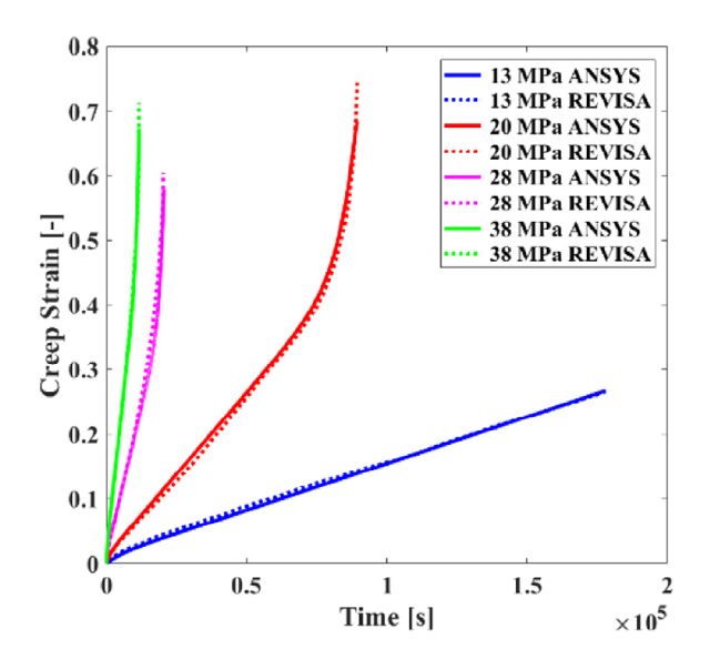
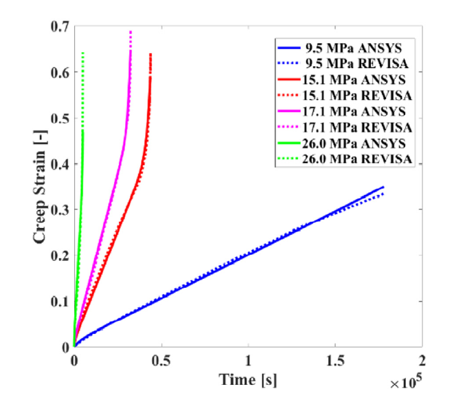


 WeChat