Global optimum of microstructure parameters in the CMWP line-profile-analysis method by combining Marquardt-Levenberg and Monte-Carlo procedures

1. Introduction

Line profile analysis (LPA) of X-ray and neutron diffraction patterns proved to be a powerful method to obtain quantitative characterization of lattice defects in crystalline materials [[1], [2], [3], [4], [5], [6], [7]]. There are two different approaches of LPA. The top-down approach is using standard profile functions like Gaussian, Lorentzian, pseudo-Voight or Pearson-VII for fitting peak profiles [[8], [9], [10]]. In this approach it is often difficult to interpret profile function parameters in terms of physical properties of the microstructure. In the Convolutional Multiple Whole Profile (CMWP) approach [4,5,7] the profile functions are based on well-established physical principles using the physical properties of specific lattice defects [3,[2], [3], [4], [5], [6], [7],[11], [12], [13], [14], [15], [16], [17]]. Size profiles are calculated on optical principles [18] and the concept of column lengths [19]. Size distribution is taken into account assuming log-normal size distribution [20]. Strain profile is calculated by using the Krivoglaz-Wilkens theory of microstrain produced by dislocations [13,14,16]. Planar defects are included by calculating the profile functions for layered structures [15,17,21]. Compatibility strains are either related to (i) strain gradients produced by geometrically necessary dislocations (GNDs) [[22], [23], [24]] or to (ii) anisotropic pure elastic strains of hard inclusions [[25], [26], [27]]. The first is captured in the strain profiles delivering the total dislocation density including the dislocation density of both GNDs and statistically stored dislocations (SSDs) [[28], [29], [30], [31], [32]]. Line broadening due to the second is caused by peak shifts of elastically anisotropic hard inclusions or phases strained below the yield point [[25], [26], [27]]. This needs additional peak profiles. Diffuse satellite peaks around and below the fundamental Bragg reflections produced by small coherent clusters are taken into account by additional peaks with appropriate hkl dependence [33].

The different physical properties of the microstructure are separated by using the differences in the hkl dependence and the shape of profiles. The relatively large number of possible physical parameters renders a serious challenge for the Marquardt-Levenberg (ML) [34,35] optimization procedure. In the parameter space there can be local minima where, depending on the initial parameter values, the optimization process can get stuck. In the present work we develop a Monte-Carlo (MC) type [36] statistical procedure and show that the combined ML plus MC optimization is independent of the initial parameter values providing the global optimum for the physical parameter values. The advanced CMWP method supporting the ML procedure by implementing a MC approach will be freely available on the web: http://csendes.elte.hu/cmwp/.

2. Principles of the convolutional multiple whole profile (CMWP) procedure

2.1. Profile functions in the CMWP procedure

The method is based on physically modeled profile functions of the different microstructural elements. The two very different microstructure elements are the size and strain effects [1]. In diffraction patterns these two combine as convolution. For a particular hkl diffraction peak:

$I_{hkl}(s)=I^{S}_{hkl}(s)^{*}I^{D}_{hkl}(s)$, (1)

where I^S and I^D are the size and strain profiles, respectively. The variable s is: s = K - g_hkl, where g_hkl is the fundamental reciprocal lattice vector of the hkl reflection and K is an arbitrary reciprocal space vector. Eq. (1) indicates that diffraction peaks are three dimensional in reciprocal space. In powder diffraction experiments the intensity distributions are integrated along the surface perpendicular to the diffraction vector, g_hkl, and Eq. (1) reduces to one dimensional:

$I_{hkl}(s)=I^{S}_{hkl}(s)^{*}I^{D}_{hkl}(s)$, (2)

where s = 2(sinθ-sinθ_B)/λ, θ and θ_B are the diffraction angle and the exact Bragg angle of the hkl peak and λ is the wavelength of radiation. The equivalent of Eq. (1) in Fourier space is:

$A_{hkl}(L)=A^{S}_{hkl}(L)·A^{D}_{hkl}(L)$ (3)

where L is the Fourier variable. If planar defects (PD), elastic compatibility strains (ECS) and instrumental effects are also present the above equation becomes:

$A_{hkl}(L)=A^{S}_{hkl}(L)·A^{D}_{hkl}(L)·A^{PD}_{hkl}(L)·A^{ECS}_{hkl}(L)·A^{Inst}_{hkl}(L)$ , (4)

where $A^{PD}_{hkl}(L)$, $A^{ECS}_{hkl}(L)$ and $A^{Inst}_{hkl}(L)$ are the Fourier transforms of the profiles corresponding to PDs, ECSs and instrumental effects, respectively. As mentioned before, the Fourier transforms $A^{S}_{hkl}(L)$, $A^{D}_{hkl}(L)$, $A^{PD}_{hkl}(L)$ and $A^{ECS}_{hkl}(L)$ are modeled by using physical properties of these lattice defects [[2], [3], [4], [5], [6], [7]] and $A^{Inst}_{hkl}(L)$ is determined by using measured patterns of defect free standard materials. The diffraction pattern is calculated from the inverse Fourier transforms of A_hkl(L):

$I_{Calc}(2θ)=\sum_{hkl}I^{hkl}_{0}FT^{-1}[A^{S}_{hkl}(L)·A^{D}_{hkl}(L)·A^{PD}_{hkl}(L)·A^{ECS}_{hkl}(L)·A^{Inst}_{hkl}(L)](2θ-2θ^{hkl}_{0})$ (5)

where $θ^{hkl}_{0}$ and $I^{hkl}_{0}$ are the exact Bragg position and the maximum intensities of the hkl reflections above the background intensity, respectively. The least-squares optimization is done by minimizing the weighted sum of squared residuals (WSSR):

$WSSR=\sum_{i}\{[I_{Calc}(2θ_{i})+BG(2θ_{i})]-I_{Meas}(2θ_{i})\}^{2}w_{i}$ (6)

where BG(2θ_i) is the background at 2θ_i and w_i is the weight corresponding to the data point i.

In CMWP the size profile is calculated by assuming spherical coherently scattering domains with lognormal size distribution [4,5,7]:

$IS(s)=\int_{0}^{∞}\frac{sin^{2}(tπs)}{(πs)^{2}}erfc[\frac{ln(\frac{t}{m})}{\sqrt{2}σ}]dt$ (7)

where m and σ are the median and the variance of the size distribution function and erfc is the complementary error function. The Fourier transform of the strain profile is:

$A^{D}_{hkl}(L)=exp(-2π^{2}L^{2}g^{2}<ε^{2}_{g,L}>)$, (8)

where $<ε^{2}_{g,L}>$ is the mean square strain. Krivoglaz has shown that strain broadening can only be caused by one dimensional linear defects [16] which are dislocations. (An exception to this case is when line broadening is caused by pure ECSs, as discussed in references [26] and [27]) With this:

$<ε^{2}_{g,L}>=\frac{ρCb^{2}}{4π}f(\frac{L}{R_{e}})$ (9)

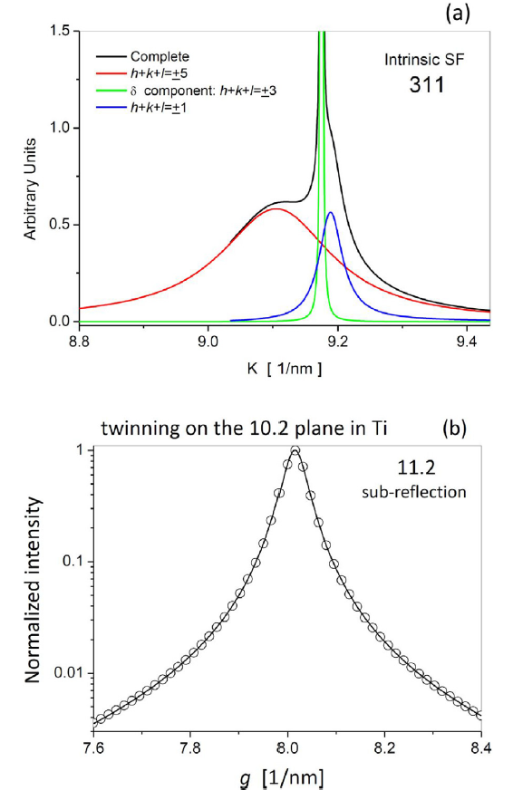
where ρ, C and b are the density, the contrast and the Burgers vector of dislocations and R_e is the effective outer cut-off radius of dislocations [14]. The actual value of R_e depends on the dislocation density. Therefore Wilkens [14] introduced the dislocation arrangement parameter M=Re$\sqrt{ρ}$. This is a dimensionless number characterizing the arrangement or the dipole-character of dislocations. Small or large M values, i.e. M about smaller or about larger than 1, mean strong or weak screening of the strain fields, as well as strong or weak dipole-character. When M is small or large the tails of peak profiles are longer or shorter, respectively [14]. The explicit form of the f $(\frac{L}{R_{e}})$ function is given in (A6) to (A8) in [14] and is shown in Fig. 1. The profile functions of faulted and twinned crystals consist of several sub-profiles [1,15,17,21]. Typical sub-profiles of the 311 reflection of copper containing 4% of intrinsic stacking faults are shown in Fig. 2(a). The number, positions and breadths of sub-profiles depend on the hkl indices of the fundamental Bragg peak [1,15,17,21,37,38]. In CMWP the shifts and breadths of the sub-profiles are parameterized as a function of the density of specific planar faults. Balogh et al. [17,21] calculated theoretical patterns of faulted crystals by using the DIFFAX software of Treacy at al. [15]. The numerically calculated sub-profiles were fitted by the sum of symmetrical and anti-symmetrical Lorentzian functions [17,21]. It was shown that the asymmetry is caused by an interference effect when the tails of two sub-profiles overlap in reciprocal space. This effect becomes observable when the two sub-profiles are close to each other in reciprocal space. A typical 11$\bar{2}$2 sub-profile for twinning on the (10$\bar{2}$2) plane of Ti is shown in Fig. 2(b) [39]. Numerically calculated asymmetrical sub-profiles fitted by the sum of symmetrical and anti-symmetrical Lorentzian functions are shown in Figure 9 of reference [39].

As mentioned before, compatibility strains in polycrystalline materials can either be related to (i) strain gradients built up by GNDs [[22], [23], [24]] or to (ii) pure elastic strains below the yield point of hard precipitates or inclusions [[25], [26], [27]]. For the first case it has been shown in several works that LPA catches both GNDs and SSDs together. For example GNDs producing long-range internal stress in dislocation cell structures [[28], [29], [30]], GND type misfit dislocations at the interface between γ and γ' phases in Ni-base superalloys [25], or the GNDs at the interphase between martensite laths and austenite layers are always included in the total dislocation densities together with the SSDs [31,32]. In the second case non-deformable, elastically strained hard particles or phases produce peak shifts [[25], [26], [27]]. Leineweber [26,27] has shown that anisotropic thermal expansion in polycrystalline orthorhombic cementite produces temperature dependent line broadening. This latter effect needs special treatment if dislocations and ECSs related line broadening occur at the same time. The model in reference [27] can provide guidelines for constructing profile functions, $I^{ECS}_{hkl}(s)$, based on the elastic constants of the hard inclusions. The $I^{ECS}_{hkl}(s)$ can be convoluted with the instrumental profile functions, $I^{Inst}_{hkl}(s)$ (s) producing effective instrumental profiles, $I^{Eff-Inst}_{hkl}(s)$. Using these modified instrumental profiles delivers the true dislocation density free from the effect of ECSs.

2.2. Physical and auxiliary parameters in the CMWP procedure

In the CMWP procedure only the microstructure parameters are considered as physical quantities. Peak positions and peak intensities are considered as auxiliary parameters. The physical parameters are (i) the dislocation density ρ, (ii) the dislocation arrangement parameter M, (iii) dislocation contrast, C and (iv) the planar fault density, α or β for stacking faults or twin boundaries. The contrast factor of dislocations depends on the relative orientation between the Burgers and line vectors, b and l, the diffraction vector, g, and the elastic constants of the crystal, c_ijkl: C=C(b,l,g,c_ijkl) [19]. In a texture free polycrystal or if all possible Burgers vectors are randomly populated, C can be averaged over the permutations of the hkls [40,41]. In the case of cubic and hexagonal crystals the average contrast factors, $\bar{C}$, can be written as [42,43]:

$\bar{C}=\bar{C}_{h00}(1-qH^{2})$, (10)

$\bar{C}=\bar{C}_{hK.0}(1+a_{1}H^{2}_{1}+a_{2}H^{2}_{2})$ (11)

where $\bar{C}_{h00}$ and $\bar{C}_{hK.0}$ are the average contrast factor for of the h00 and hk.0 type reflections in cubic and hexagonal crystals, respectively. The hkl dependence in cubic and hexagonal materials is given by the H²=( h²k²+ h²l²+k²l²)/( h²+k²+l²)² and the

expressions [4,42,43]. The q, and a₁ and a₂ are the physical parameters providing the dislocation contrast factors for cubic and hexagonal crystals, respectively. The CMWP procedure allows evaluating diffraction patterns consisting of more than one phase. In such cases the number of physical parameters increases. In the simplest case of a cubic single phase material with spherical crystallite shape and no planar defects the number of physical parameters will be five: ρ, M, and q for the strain profile and m and σ for the size profile. In an hcp specimen, containing two different phases, the number of physical parameters becomes twelve: ρ, M, m, σ and a₁, a₂, and ρ¹, M¹, m¹, σ¹ and $a^{1}_{1}$, $a^{2}_{1}$, where the upper index 1 is for the second phase.

2.3. Algorithms used for solving equation (6)

Eq. (6) requires solving of a non-linear problem with correlations between the different parameters. The possibilities are: (a) nonlinear least-squares algorithms [44], (b) direct search methods [43,45] and (c) statistical methods [36]. Within the nonlinear least-squares algorithms there are the Newton-method, the steepest descent method and the (ML) [34,35] methods. The non-linear least-squares algorithms provide the local minimum by definition. Nonlinear least-squares algorithms cannot guarantee the equivalence of the global and local minima. The global minimum is found by the successive application of an MC [36] type and the ML algorithms. We developed the following MC procedure for CMWP. The fitting parameters are only the physical parameters: q, m, σ, ρ and M for cubic or a₁, a₂, m, σ, ρ and M for hcp materials. Based on physical considerations each parameter is restricted between a minimum and maximum value which cannot be bypassed. However, the minimum/maximum restrictions can be edited freely by the user. In consecutive iterations the new parameter values are searched in the proximity of the previous ones:

$a^{i}_{n}∈[a^{i}_{n-1}+Δ^{i}_{n};a^{i}_{n-1}-Δ^{i}_{n}]$ (12)

This means that i is the parameter index and n is the current iteration number. Δni is defined as:

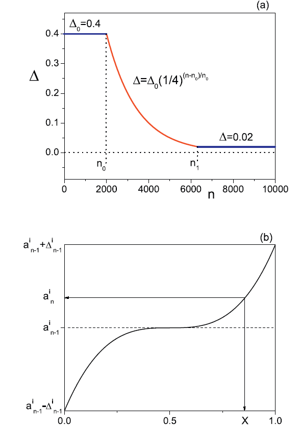
where $Δ^{i}_{n}$ remains unchanged during the first n₀ iterations. In the following iterations $Δ^{i}_{n}$ is reduced to Δmini. Once Δni reaches $Δ^{i}_{min}$, the $Δ^{i}_{n}$ values are kept constant. The Δ(n) function, as shown in Fig. 3(a), is decaying between n₀ and n₁ as: Δ=Δ₀ $a^{(n-n_{0})/n_{0}}$, where a=$(Δ^{i}_{min}/Δ_{0})^{n_{0}(n_{1}-n_{0})}$. From this equation the value of n₁ will be n₁ = 6322 if n₀ = 2000, Δ₀ = 0.4, Δ_min = 0.02 and a = 1/4, as in Fig. 3(a). (For simplicity the superscript i has been omitted here.) It is noted, however, that the parameters for the fitting conditions, especially: Δ₀, Δ_min and n₀ can be edited freely by the user. We also note that the actual values of Δ₀ and Δ_min do not influence the optimization procedure substantially. Experience has shown that varying these two values within a wide range around the default ones, i.e. around Δ₀ = 0.4 and Δ_min = 0.02, did not affect the global optimum results. It is also noted that the actual functional form of the decay of $Δ^{i}_{n}$ in Eq. (13b) is not critical. Different functional forms of the decay will lead to the same global optimum. For the consecutive iterations a bias towards the prevailing parameter value, $a^{i}_{n-1}$ is implemented using a cubic probability function for the deviation of the consecutive parameter values, $a^{i*}_{n}$:

$a^{i*}_{n}=Δ^{i}_{n}·(2x^{i}_{n}-1)^{3}+a^{i}_{n-1}$ (14)

where the value of $x^{i}_{n}$∈0,1 is given by a random number generator. The star in $a^{i*}_{n}$ indicates that this consecutive value has not yet been accepted as a better value than an-1i. A schematic relation between the random generated number, $x^{i}_{n}$, and the consecutive parameter value on the biased cubic probability (BCP) function is shown in Fig. 3(b). The purpose of the BCP function is sampling the parameter space on a finer scale around the preceding values. However, as it can be seen on the BCP curve, there is a good chance of sampling remote regions in the parameter space as well. The condition for accepting the new parameters, $a^{i}_{n}$ is:

$a^{i}_{n}=\{\mathop{}_{a^{i}_{n-1},if\ \ WSSR_{n}≥WSSR_{n-1}}^{a^{i*}_{n},if\ \ WSSR_{n}<WSSR_{n-1}}\}$ (15)

The errors of the parameter values are determined in terms of p% fractions of the WSSR. If a particular WSSR value is larger than the best value, WSSR_best, found until the actual iteration, but within a certain p% fraction of WSSR_best, i.e.

WSSR>WSSR_best AND WSSR<(1+ p%)·WSSR_best, (16)

then the parameter values corresponding to WSSR=(1+ p%)·WSSR_best will be the instantaneous plus-minus errors of the parameters. The convergence criteria in our MC procedure are that (i) the number of steps has to reach a user defined value, i.e. the "MC_min_steps" value defined by the user in the frontend and (ii) the 1+p% statistics has to be at least N_p. The second criterion means that among all the iterations at least N_p were such that the WSSR was not larger than the last (1+ p%)·WSSR_best value. The systematic testing of the combined ML + MC algorithm has shown that n₀ = 2000, p = 3.5% and N_p = 100 give excellent pattern fittings and good physical parameter values even if the diffraction patterns are complicated [46]. The combination of ML and MC algorithms in CMWP are organized in the following manner. It is assumed that the initial values of peak positions and peak intensities are determined correctly. Optimization starts with the MC algorithm where only the physical parameters as defined in paragraph 2.2 are refined. In the ML algorithm the physical parameters are refined along with the peak positions and peak intensities. The optimization procedure ends when the MC algorithm reached the number of steps, N_p within which the WSSR did not exceed (1+p%)⋅WSSR and the ML algorithm converged.

2.4. Extension of CMWP for handling satellites or diffuse scattering

Guinier-Preston (GP) zones [47], small dislocation loops [48] or diffuse scattering of solute atoms [49] can produce satellites or diffuse scattering peaks around or below the fundamental Bragg peaks. The evaluation of the dislocation density and arrangement relies strongly on the lower intensity regions of strain profiles. Satellites or diffuse scattering peaks not related directly to the strain profiles but rather to strain fields around small coherent GP zones, dislocation loops or solute atoms may distort the physical parameter values obtained from the lower intensity regions of diffraction peaks. CMWP provides the option to treat such low intensity diffuse scattering type intensity modulations in a systematic manner using a limited number of global parameters for the entire diffraction pattern. It is assumed that the satellites or diffuse scattering stem from strain fields around small coherent volumes and are fitted by Pearson-VII profile functions shifted by Δ(2θ)=s₀g $\sqrt{\bar{C}}$ relative to the corresponding Bragg peaks. The contrast, $\bar{C}$, depends on the strain fields related to the small coherent objects producing the satellites or diffuse scattering. The value of s₀ is a global parameter for all the peaks in the entire pattern. During the optimization procedure the Pearson-VII profile functions are added to the background spline. This procedure has been applied to evaluate satellite peaks produced by small dislocation loops in proton or neutron irradiated Zr alloys [33].

2.5. Stabilizing the fluctuations of the physical parameters when the effective outer cut-off radius, R_e, approaches the lower limit of continuum theory

A systematic investigation of the f(η) function revealed that when M drops into the range around or below unity along with large dislocation densities in the range of 10¹⁶⋅ m^-2 the effective outer cut-off radius, R_e, can reach small values of a few nm. Such R_e values approach the lower limit of continuum theory not far from atomic distances [50,51]. In neutron [52] or proton [53] irradiated Zr alloys the dislocation line density can reach a few times 10¹⁶⋅ m^-2 while the M value is around M≅1 or smaller. With these values R_e≅2 to 4 nm. In the corresponding diffraction patterns the profiles broaden mainly in the lower intensity range while the full width at half maximum (FWHM) stays almost unchanged, see e.g. Fig. 8(a) in reference [53] or in Fig. 1(b) in reference [33]. In the Krivoglaz-Wilkens strain function (see Eq. (9)) ρ and M are determined from the logarithmic part of f(η) [3,13,14,16]. If R_e becomes extremely small the logarithmic part of f(η) shrinks to a short section, as it can be seen in Fig. 1 (see the double-dot dash line), and the values of R_e and ρ might reveal some instability. In order to avoid the degenerate behavior of R_e we introduced a lower limit, R_c for R_e by replacing η=L/R_e by η=L/(R_e+R_c). We have shown that whenever R_e is larger than R_c then the value of R_c becomes irrelevant. Introducing R_c, however, prohibits R_e to become unrealistically small. The effect of R_c on the values of ρ and M has been investigated systematically by evaluating the diffraction pattern of a proton irradiated Zircaloy-2 specimen [33] (see Fig. 1(c) in reference [33]). Fig. 1(c) in reference [33] shows that the values of ρ and M are fairly stable and robust for R_c between about 4 and 8 nm: 4≤R_c≤8 nm. The selection of R_c in the range between 4 and 8 nm is justified by the lower limit of lengths in continuum theory [50,51]. The Krivoglaz-Wilkens theory of strain broadening is based on continuum theory [3,13,14,16]. When ρ becomes larger than about 10¹⁶⋅ m^-2 along with M dropping to 1 or lower, R_e approaches the lower limit of the lengths in continuum theory [50,51]. The introduction of R_c protects R_e to enter a length region illegal in the continuum approach. To date there is no better strain function than f(η). Practically this also justifies the introduction of R_c. Renormalizing the Krivoglaz-Wilkens function by introducing R_c makes determining the physical parameters in CMWP more robust and reliable even for extreme values of ρ and M.

2.6. Modification of the ML algorithm in the gnuplot program package

The ML code of CMWP is based on the ML code implemented in the gnuplot program package. Sometimes the original ML code of gnuplot did not change significantly the value of the ρ parameter and its value was stuck near its initial value. The following modification of this code significantly improved the convergence of ρ. In each step of the ML procedure the parameter values are modified by a value calculated as the partial derivative of chi-square as a function of the parameter in question multiplied by a common step Lambda, which is changed adaptively during the algorithm. Only in the case of the ρ parameter the modified algorithm tries first to change the value of ρ - in the same direction as the original algorithm would do - by a larger value, e.g. by 10% and 2%. If either of these trials is successful (e.g. the value of WSSR is decreased) then the new value of ρ is accepted. If not, then its value is changed as the original algorithm calculated it. This way, the modified ML code approaches the minimum with larger steps and works significantly better compared to the original code.

3. Testing the combined ML + MC optimization in the CMWP procedure

3.1. Testing the combined ML + MC optimization procedure on two difficult diffraction patterns

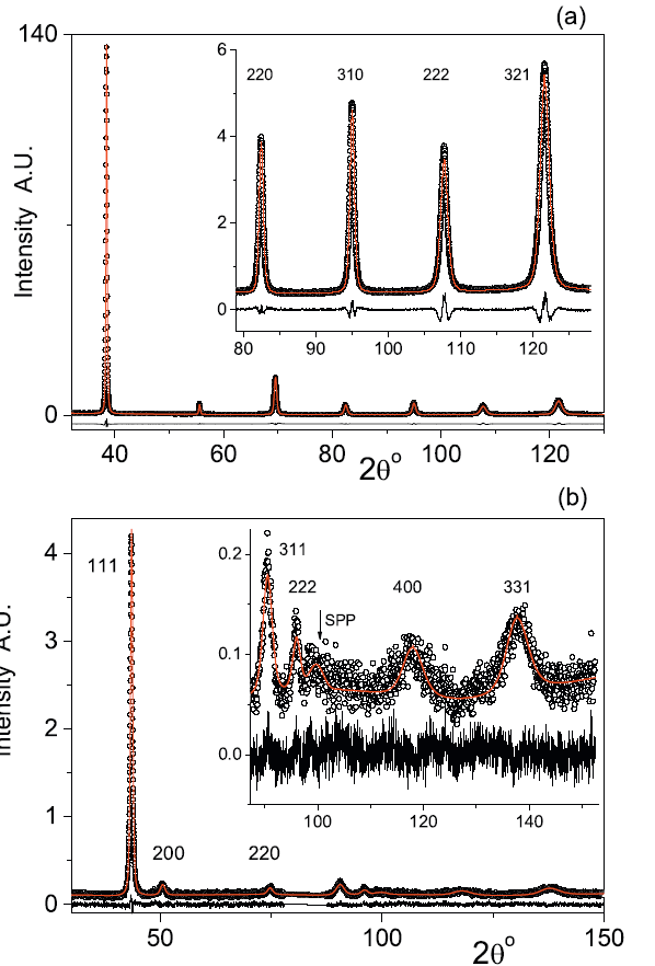
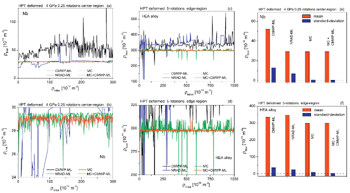
We are testing the combined ML + MC optimization in the CMWP procedure on the diffraction patterns of (a) pure Nb high pressure torsion (HPT) deformed at 4 GPa and 0.25 rotations [54] and (b) a Cantor [55] type high-entropy-alloy (HEA) HPT deformed at 4 GPa and 5 rotations [56]. The diffraction patterns are shown in Fig. 4. The open circles are the measured and the red solid lines the CMWP calculated patterns. The black lines in the bottom of the figures are the difference between the measured and calculated patterns. CMWP has been systematically run on the two diffraction patterns by starting with initial dislocation density values, ρ_initial in the range of 1-300 [10¹⁴ m^-2] for the Nb and in the range of 1-1000 [10¹⁴ m^-2] for the HEA patterns, respectively. Four optimization algorithms have been tested. (i) $\ddot{C}$MWP-ML $\ddot{t}$he ML algorithm in the modified gnuplot program package in a linux platform (this is used in the CMWP procedure). (ii) $\ddot{N}$RAD-ML$\ddot{:}$ an ML algorithm based on the handbook of Numerical Recipes [57] where the derivatives of the physical profile functions have been calculated analytically. (iii) $\ddot{M}$C$\ddot{t}$he CMWP procedure when only the MC algorithm is used. (iv) $\ddot{M}$C + CMWP-ML$\ddot{t}$he combination of (i) and (iii) as it is in the CMWP procedure with the combined ML and MC algorithms. Fig. 5(a) and (c) show the final dislocation densities, ρ_final as a function of ρ_initial obtained by using the four optimization procedures. For better seeing the two MC algorithms the ρ_final scale is enlarged in Fig. 5(b) and (d). The figures show that the best results are obtained by MC + CMWP-ML algorithm implemented in the new CMWP procedure. The statistics on the evaluation procedures are shown in Fig. 5(e) and (f) for the two patterns. Both figures show that the means are very close to each other when MC algorithm is implemented and the smallest standard-deviation values are obtained when the MC + CMWP-ML algorithm is applied.

3.2. Correlation between dislocation densities determined by electron microscopy and line profile analysis

Dislocation densities can vary over a wide range. To date 10 inch Si wafers are produced free of dislocation, cf. [58]. In as-quenched lath martensite steels the dislocation densities are between 10¹⁵ and 10¹⁶ m^-2 [59]. In cyclically deformed cell forming materials the dislocation densities in the cell walls of persistent slip bands become larger than 10¹⁶ m^-2 [53]. When the average dislocation distance becomes larger than about 2 μm, i.e. ρ ≤ 2.5 × 10¹³ m^-2, and the grain size is also larger than 2 μm, X-ray scattering enters the dynamic scattering regime and kinematical line broadening becomes irrelevant [18]. When the local dislocation distance becomes smaller than about 20 nm, i.e. ρ ≥ 2.5 × 10¹⁵ m^-2, the transmission electron microscopy (TEM) dislocation contrasts overlap and dislocation density determination by TEM becomes difficult [60,61]. The TEM micrograph in Fig. 1 of reference [60] shows that in cyclically deformed Cu single crystals it is practically impossible to determine the dislocation density in the cell walls of persistent slip bands. The correlation between TEM and LPA determined dislocation density has been checked in the range between ρ≅2.5 × 10¹³ m^-2 and ρ≅1 × 10¹⁵ m^-2 in references [[62], [63], [64], [65], [66], [67], [68]]. Within this range the dislocation density values provided by TEM and LPA were found to be in very good correlation. LPA is not restricted when ρ is larger than 1 × 10¹⁵ m^-2. This makes it one of the most reliable methods to determine large dislocation density values.

4. Conclusion

We extended the CMWP X-ray and neutron diffraction line profile analysis procedure to provide the global optimum of microstructure parameters in crystallite materials. The procedure is based on well-established physical models of profile functions for strain, size and planar defects. Provision has been implemented for satellite peaks around fundamental Bragg reflections and diffuse scattering below Bragg peaks. The procedure is using the numerical Marquardt-Levenberg and a statistical Monte-Carlo algorithm alternating successively. Physical parameters related to strain, size and planar defects are optimized by both algorithms. The Marquardt-Levenberg algorithm is used to optimize the physical parameters along with all auxiliary parameters not directly related to the microstructure, e.g. peak positions and peak intensities. The efficiency of implementing the Monte-Carlo algorithm into CMWP has been tested by varying the initial values of dislocation densities over a wide range in two specific examples.

Acknowledgements

G.R. gratefully acknowledges the support of the János Bolyai Research Fellowship of the Hungarian Academy of Sciences. T.U. is grateful for partial funding of this work by an EPSRC Leadership Fellowship [EP/I005420/1, EP/K039237/1, EP/K034650/1, EP/L018616/1 and EP/K034332/1] for the study of irradiation damage in zirconium alloys.

The authors have declared that no competing interests exist.

---