


Analytical Description for Solid-State Phase Transformation Kinetics: Extended Works from a Modular Model, a Review
[Feng Liu*  , Kai Huang, Yi-Hui Jiang
* , Shao-Jie Song, Bin Gu]
, Kai Huang, Yi-Hui Jiang, Shao-Jie Song, Bin Gu]
|
|


Solid-state phase transformation plays an important role in adjusting the microstructure and thus tuning the properties of materials. A general modular, analytical model has been widely applied to describe the kinetics of solid-state phase transformation involving nucleation, growth and impingement; the basic conception for iso-kinetics which constitutes a physical foundation for the kinetic models or recipes can be extended by the analytical model. Applying the model, the evolution of kinetic parameters is an effective tool for describing the crystallization of enormous amorphous alloys. In order to further improve the effectiveness of this kinetic model, recently, the recipes and the model fitting procedures were extended, with more factors (e.g., anisotropic growth, soft impingement, and thermodynamic driving force) taken into consideration in the modified models. The recent development in the field of analytical model suggests that it is a general, flexible and open kinetic model for describing the solid-state phase transformation kinetics.
Since the microstructure of metals and alloys is often changed by deliberately generated solid-state phase transformations to meet the performance requirements, much effort has been spent on modeling solid-state phase transformation kinetics[1, 2, 3, 4, 5, 6, 7, 8, 9], which concerns itself with the paths and rates adopted by the systems from initial to final states. For most solid-state phase transformations in metals and alloys, the kinetic path can be subdivided into three overlapping mechanisms: nucleation, growth and impingement. Therefore, an exact description of the kinetics of solid-state phase transformation involving the above-mentioned three mechanisms is of great importance to both scientific interests and engineering applications.
The differential scanning calorimetry (DSC) and dilatometry (DIL) are often adopted to investigate the solid-state phase transformation kinetics experimentally, providing direct information about transformation rate, df/dt or df/dT, (from DSC) and transformed fraction, f, (from DIL). Since the experimental results contain the combined effect of nucleation, growth and impingement, the formal kinetic theory focuses on analytically predicting the evolution of overall kinetic information with time, t, (isothermal case with constant annealing temperature) or temperature, T, (non-isothermal case with constant heating/cooling rate). In typical treatments, the Kolmogorov-Johnson-Mehl-Avrami (KJMA) equation[1, 2, 3, 4, 5] is an original theory for describing the isothermal transformation. However, researchers favor non-isothermal annealing in experiments and industry applications, and have concluded KJMA-like equation[11, 12]. The physics basis for the KJMA-like equation was recognized the same as the original KJMA equation until a path variable was introduced [7, 8]. In KJMA (-like) model, the iso-kinetic transformation was defined, i.e., if the transformation mechanism was invariant during the whole range, the kinetic parameter (i.e., Avrami exponent, n, overall effective activation energy, Q, and pre-exponential factor of rate constant, K0) would remain constant. Therefore, these models can be valid only when all the kinetic parameters, t(isothermal) or T (non-isothermal), remain constant. However, in practice, the kinetic parameters generally depend on t/T, causing classical models invalid. Accordingly, a general, flexible, modular analytical model with variable kinetic parameters (i.e., n(t), Q(t), K0(t) for isothermal case; n(T), Q(T), K0(T) for non-isothermal case) was proposed [13]. In the analytical model, the basic conception for iso-kinetic transformation was extended, i.e., even if transformation mechanism keeps constant during the entire transformation, the kinetic parameters do not have to be constant[14]. This model has been applied successfully to the crystallization of many amorphous alloys, which suggests that the analytical model can effectively describe the solid-state phase transformation kinetics.
In order to exploit this analytical model to its full extent, vigorous development has been carried out recently from the following aspects. (i) Several kinetic analysis recipes for extracting more crucial kinetic information (e.g., impingement mode, activation energies for nucleation and growth) from experimental data were proposed. (ii) In the framework of analytical model, the expressions for kinetic parameters were modified for describing the transformations with complicated mechanisms (e.g., transformation with sufficiently high value of initial transformation temperature, and transformations due to multi-processes). Additionally, modified analytical model extended the scope of “ iso-kinetics” . (iii) Inspired by the modular analytical model, researchers took two important factors— soft impingement and anisotropic growth— into consideration, and revealed that the evolution of transformed fraction and kinetic parameters were strongly influenced by the two factors. (iv) Chemical and mechanical driving forces were coupled into the analytical model, yielding more reasonable explanations for many kinetic phenomena appearing in the vicinity of equilibrium state.
The present paper intends to review the latest development in the field of analytical model.Section 2 describes several methods for experimentally investigating solid-state phase transformation. Section 3 briefly introduces a theoretical background essential for the analytical models. Section 4 presents the derivation and application of new kinetic recipes based on the analytical model. Section 5 summarizes the modification and application of analytical model. Section 6 discusses the effects of soft impingement and anisotropic growth. Section 7 evaluates the effects of thermodynamic factors. Section 8 summarizes the paper with prospects into the future.
The solid-state phase transformations involved in this review can be mainly divided into two subjects: the crystallization of amorphous alloy and the solid-state phase transformation in Fe-based alloys. The two kinds of transformations exhibit different features, which require varied experimental techniques to investigate their kinetics, e.g., the DSC experiment was often used to detect the crystallization kinetics, while the DIL experiment was applied to measure the phase transformations in Fe-based alloys.
Master alloys were generally obtained by melting pure elements in an induction furnace or an arc melting furnace under the inert gas atmosphere (e.g., argon). Then amorphous alloy was prepared from the master alloys by melt spinning (e.g., for Fe40Ni40P14B6amorphous alloy), injection cast into a copper mold (e.g., for Zr46Cu46Al8 amorphous alloy) or water quenching (e.g., for Pd40Cu30P20Ni10 amorphous alloy). Then specimens used for DSC experiment were cut from the amorphous material. As for DIL specimens, the Fe-based master alloy was first hammered, then it was annealed at a high temperature (e.g., 1473 K for Fe-Mn and Fe-Co alloys) for a long time (e.g., 100 h for Fe-Mn and Fe-Co alloys), and finally it was machined to cylindrical DIL samples in certain sizes (e.g., for Netzsch DIL 402C, the standard sample is 25 mm in length and has a diameter of 6 mm).
2.2.1. Differential scanning calorimetry
The crystallization kinetics was investigated by DSC scan (e.g., Perkin Elmer or Netzsch), employing a protective gas atmosphere of pure inert gas (e.g., nitrogen or argon). The temperature and the heat flow were calibrated by measuring the melting points and the heats of fusion of pure metal (e.g., In, Pb and Sn). The baseline corrections were performed according to the recipe described in Reference 8. Two identical DSC run were made successively for each sample. The second run with the specimen in its crystalline state served as an in situ recording of the baseline. And the measurement curve was obtained by subtracting the baseline from the first run. Then, the enthalpy change curves obtained from the DSC experiment can provide the kinetic information about transformation rate.
2.2.2. Dilatometry
The solid-state phase transformation in Fe-based alloy was measured by DIL (e.g., Netzsch DIL 402C), with fresh specimen for each measurement. The measurements were performed under flowing argon to prevent the specimens from oxidization. The temperature was calibrated, and baseline correction was also performed. In the first run, the length change of the standard Al2O3 sample was measured, which served as a reference line. In the second run, the length change of Fe-based alloy specimen was measured, and then the measurement curve was obtained. Accordingly, the evolution of transformed fraction can be obtained from the length change curves obtained from the DIL experiment.
The present paper mainly focuses on the transformation kinetics involving nucleation, growth and impingement. The formation of supercritical particle of new phase in matrix of parent phase is called nucleation, during which phase interfaces develop between the new and the parent phases. Growth corresponds to the interface movement from the new phase toward the parent phase. Yet impingement describes the interactions among new-phase grains upon growth. Generally, the three mechanisms can be modeled separately. In the following, a number of nucleation, growth and impingement modes are discussed respectively, followed by the overall phase transformation kinetic models.
3.1.1. Continuous nucleation
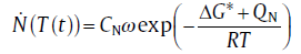
The rate of nucleation is determined by the number of particles with critical size and the jumping rate of atoms through the phase interface between the parent phase and the critical particles. The classical nucleation theory (CNT), which was formulated for the condensation of pure vapor to form liquid[15], can be modified for describing the nucleation rate in solid-state[16]:
 (1)
(1)
where R is the gas constant, T the temperature, CN the number density of suitable nucleation sites, ω the characteristic frequency factor, Δ G* the critical energy barrier for nucleation and QN the activation energy for nucleation. In this paper, the nucleation process which can be described by the CNT is termed as continuous nucleation.
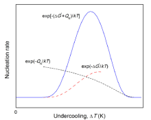
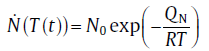
Since Δ G* depends on temperature, the nucleation rate described by Eq. (1) changes dramatically with the undercooling, Δ T (=Te-T, with Te as the equilibrium temperature) (see Fig.1). If Δ T is large enough (i.e., for the extremely non-equilibrium state), Δ G* is so small that it can be neglected as compared to QN, and Eq. (1) is reduced to an Arrhenius relationship[8]:
 (2)
(2)
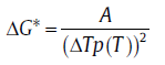
where N0 is the constant nucleation rate. However, with Δ T decreasing, the influence of Δ G* increases gradually, and the nucleation rate deviates from the Arrhenius relationship. It even shows an anti-Arrhenius behavior in the near-equilibrium state, i.e., the nucleation rate increases with T decreasing (see Fig.1)[17]. In this case, Δ G* can be expressed as a function of Δ T:
 (3)
(3)
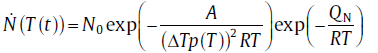
where p(T) can be expressed as 1, T/Te, 2T/(Te+T) and 7T/(Te+6T), respectively, according to different authors [18, 19, 20], and A represents the model parameter related to the interface energy, the geometric constant of the nucleus, the enthalpy change during phase transformation and Te. Substituting Eq. (3) into Eq. (1), the rate of continuous nucleation in the near-equilibrium state can be expressed as[21],
 (4)
(4)
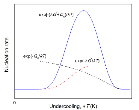 | Fig.1 Schematic diagram of the evolution of nucleation rate with undercooling. |
3.1.2. Site saturation
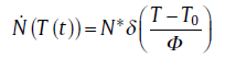
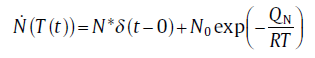
In many alloy systems with heterogeneous nucleation, nucleation only occurs in the early stage of reaction. This may be due to the limited amount of preferential nucleation sites, e.g. the grain boundaries, edges or corners in polycrystalline materials and “ frozen in” particles of crystalline phase in metallic glass, which can be consumed very early in the transformation. This effectively leads to a zero nucleation rate for the remainder of transformation. The term site saturation[6] can be applied to general case of pre-existing nuclei at T= 0 and the further nucleation rate is zero. This implies for the nucleation rate [8]:
for isothermal transformation
 (5a)
(5a)
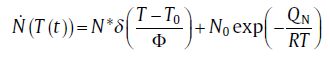
and for non-isothermal transformation
 (5b)
(5b)
where N* stands for the number of nuclei per unit volume, δ for Dirac functions with Φ as the constant heating rate (positive value) or cooling rate (negative value), T0
3.1.3. Avrami nucleation
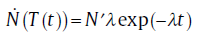
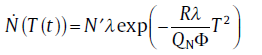
Another type of nucleation mode is named after Avrami who first described the condition in 1939[2]. In this case, the supercritical nuclei formed from the subcritical germ nuclei, Nsub, so the total number of sub- and supercritical nuclei, N′ , is constant. The change of the number of supercritical nuclei depends not only on the rate, λ , at which an individual subcritical size becomes supercritical nuclei, but also on Nsub, which decreases with the progress of transformation[13]:
where the rate λ follows an Arrhenius-type equation:
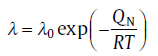 (7)
(7)
with λ 0 as a constant. Upon integration of Eq. (6), after separation of variables, using Eq. (7) and the boundary condition that the number of subcritical particles clusters is zero at T= 0, the Avrami nucleation rate is obtained as follows [13]:for isothermal transformation
 (8a)
(8a)
and for isochronal transformation
 (8b)
(8b)
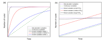
By varying N′ and/or λ , the mode of nucleation can be varied from site saturation to continuous nucleation, e.g., if λ is infinitely large, the subcritical germ nuclei become supercritical totally at the very beginning of transformation, and the nucleation mode approaches the site saturation; on the contrary, if λ is infinitely small, the number of subcritical germ nuclei can be assumed as a constant during the transformation, and the nucleation mode approaches the continuous nucleation (see Fig.2). Clearly, if these two extreme cases do not occur, the nucleation rate decreases gradually with the progress of transformation. Note that the principal difference between continuous nucleation and Avrami nucleation is that the nucleation site of continuous nucleation is invariant during the whole transformation, while that of Avrami nucleation (i.e., Nsub) is consumed gradually.
3.1.4. Mixed nucleation
In practice, mixed nucleation occurs when a number of pre-existing nuclei is present and other nuclei form during the transformation. The term mixed nucleation represents a combination of site saturation and continuous nucleation modes. In this case, the nucleation rate is equal to some weighted sum of the nucleation rates according to continuous nucleation and site saturation [13]:for isothermal transformation
 (9a)
(9a)
and for non-isothermal transformation
 (9b)
(9b)
where N* and N0 include the relative contributions of the two modes of nucleation. Similarly, by varying N0/N* , the mode of nucleation varies accordingly from pure site saturation (for infinitely small N0/N* ) to pure continuous nucleation (for infinitely largeN0/N* ) (see Fig.2(b)).
 | Fig.2 Schematic diagram of the number of nuclei as a function of time at constant temperature for (a) Avrami nucleation and (b) mixed nucleation. |
The growth of new-phase particles can be controlled by diffusion process prior to phase interface or by atomic jump process at the phase interface, yielding diffusion-controlled growth and interface-controlled growth respectively[22]. For the diffusion-controlled growth, the motion of the interface requires the long-range transport of atoms toward or away from the growing region, and the growth rate is then determined almost entirely by the diffusion conditions. On the contrary, the rate of interface-controlled growth is determined by atomic jump processes in the immediate vicinity of the interface if there is no change of composition across the interface, and the growth rate depends on both driving force and the mobility of the interface. The diffusion-controlled and interface-controlled growth modes can be described in a compact form. At time t, the volume Y of a growing particle nucleated at time τ is given by [14]
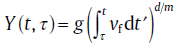 (10)
(10)
with g as a particle geometry factor, d the dimensionality of the growth (d = 1, 2, 3), mthe growth mode parameter (interface-controlled growth: m = 1; diffusion-controlled growth: m = 2), and vf the growth factor (interface-controlled growth: vf stands for growth velocity, v; diffusion-controlled growth: vf stands for the diffusion coefficient, D).
For interface-controlled growth, the growth velocity can be expressed as[14]
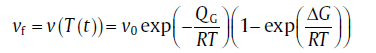 (11)
(11)
where v0 is the pre-exponential factor for growth, QG the activation energy for the transfer of atoms through the old/new phase interface and Δ G the energy difference between the new and the parent phases (Δ G is negative; the driving force for growth is defined by -Δ G). Further derivation leads to [21]
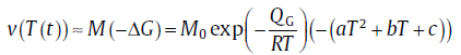 (12)
(12)
with M as the interface mobility and M0 the pre-exponential factor. For the transformation occurring in the near equilibrium state, the value for Δ G can be obtained from the thermodynamic evaluation, and the values for a, b and c are determined by a polynomial fitting; whereas if the transformation occurs in the extremely non-equilibrium state, we get a = b = 0 and c = -v0/M0 directly.
For diffusion-controlled growth, long distance diffusion in the matrix governs the growth of the new phase particles. In the extreme non-equilibrium state, according to the parabolic growth law, the radius of particle, rp(t), nucleated at time τ can be expressed as [8]
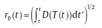 (13)
(13)
where the diffusion coefficient depends on temperature according to
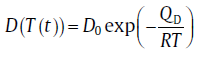 (14)
(14)
with D0 as the pre-exponential factor and QD the activation energy for diffusion. If Eq.(13) holds, the volume of the growing particle is given by
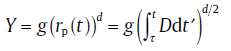 (15)
(15)
Compared with Eq. (10), the function yields vf = D. In this case, the growth behavior depends only on the diffusion coefficient. But, in the near-equilibrium state, the growth velocity is governed by both the “ supersaturation” and the diffusion coefficient [23]. In combination with a diffusion profile, C, which is a function of position and time, the growth velocity has been given by Zener as [24]
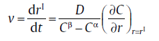 (16)
(16)
where r is the position, rI represents the position of the interface front, Cβ and Cα the equilibrium solute concentration of new phase β and parent phase α , respectively.
For diffusion-controlled growth, the assumption adopted here is that the interface mobility is infinite and the diffusion process is rate-determining. On the other hand, if the diffusivity is infinite, the rate of transformation of the lattice is determined by the velocity of the interface between the parent and the new phases, which corresponds to the interface-controlled growth. In general, neither the interface mobility nor the diffusivity will be infinite, therefore the phase transformation will be situated in between the extremes of diffusion-controlled and interface-controlled[25] (see Fig.3).
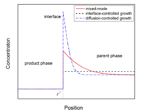 | Fig.3 Schematic diagram of the solute concentration profiles around the phase interface[25]. |
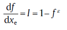
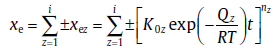
It is supposed that each nucleation takes place and every particle grows into an infinitely large parent phase, in the absence of other growing particles. In this hypothetical case, the volume of all particles is called the extended volume, which corresponds to the extended transformed fraction, xe. To account for the overlap of growing particles, researchers employ the impingement mode to describe the relationship between the real transformed fraction and the extended one.
There are two key assumptions in the derivation of original KJMA equation[1, 2, 3, 4, 5]: the nuclei distribute randomly in space and the growth rate is isotropic. Accordingly, the volume that each particle can grow into is proportional to the fraction that has not been transformed. Therefore, it is possible to deduce a quantitative relationship between f and xe, and to obtain the classical KJMA equation:
 (17a)
(17a)
If the new-phase particles grow anisotropically, fast-moving interfaces can impinge on slow-moving interfaces. It means that areas that could be transformed by the fast-moving interface, if not stopped, are effectively ‘ shielded’ by the blocking particle. Such blocking mechanism will cause severer impingement than the case of isotropic growth. Such deviation from the KJMA assumptions will influence later stages of the reaction where it will cause an additional reduction on transformation rate, and the following equation gives a good approximation for this case[14, 26]:
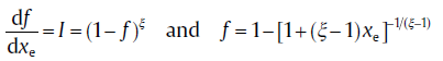 (17b)
(17b)
with ξ as an impingement factor.
In practice, nucleation may occur preferentially in certain macroscopic regions (e.g., grain boundaries), so that the nucleation probability becomes dependent on the coordinates. In this case, the KJMA assumption of random dispersed nuclei becomes invalid, i.e. Eq.(17(a)) fails to treat non-randomly dispersed nucleation. As such, a less severe impingement occurs than the case of random distribution of nuclei. The relation can thus be described as[27]
 (17c)
(17c)
with ε as another impingement factor. Note that, according to Eq. (17(c)), the specific analytical relation between f and xe does not exist, but a simple recursive procedure can be performed to calculate f from xe[14].
The above three cases deal with hard impingement, where the nucleation and growth proceed at the same rate in the untransformed region. However, in some diffusion-controlled transformations, a solute-depletion zone develops around a growing particle in which zone it is less likely, if not impossible, for further nucleation to take place, and the growth rate will be affected by the overlapping diffusion fields. This is called soft impingement. The treatment for this case is more complicated than that for the hard impingement (see section 6.1). In addition, the impingement modes for non-randomly dispersed nucleation and anisotropic growth are considered separately. Actually, these two impingement modes often take place simultaneously, for example, the nucleation of ferrite tends to occur at grain boundary and the consequent growth may be anisotropic. Up to now, there is no specific model incorporating these two cases simultaneously. So, the combined effect of the two impingement modes on the overall transformation should be addressed in future work.
Assuming that nuclei are randomly distributed and the isotropic growth rate are the same for all nuclei, the original KJMA theory gives[28]
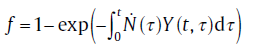 (18)
(18)
Under isothermal conditions, the nucleation rate as well as the growth rate can be considered constant for the integration in Eq. (18). By substituting Eqs. (2) (or (5(a))), (10)and (12) into Eq. (18), the integrals in Eq. (18) can be solved directly[8]:for continuous nucleation
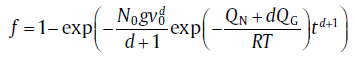 (19a)
(19a)
for site saturation
 (19b)
(19b)
Eqs. (17(a)) and (17(b)) can be summarized in a compact form
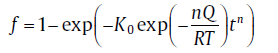 (20)
(20)
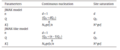
For the specific expressions of kinetic parameters, see Table 1. Eq. (20) is a basic equation in the KJMA theory, which has been widely applied in describing the evolution of transformed fraction with time.
| Table.1 Expressions for the growth exponent, n, the overall activation energy, Q, and the pre-exponential factor of rate constant, K0, to be inserted in Eq. (20) for the classical JMAK model, and in Eq. (21) for the JMAK-like model, respectively |
However, the assumptions of original KJMA model are often violated. Therefore, much effort has been spent relaxing the assumptions in the classical KJMA theory. Primarily, the non-isothermal condition, in particular, with a constant heating rate, Φ = dT/dt(isochronal), is more favorable than the isothermal condition in practice. In this case, by applying a rough approximation to the so-called “ temperature integral” , we may obtain an expression for transformed fraction [8]
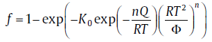 (21)
(21)
For the specific expressions of kinetic parameters, see Table 1. Eq. (21) has a similar form with the KJMA equation (i.e., Eq. (20)), so it is termed as “ KJMA-like” equation. However, the physical basis of the similarity between the KJMA and the KJMA-like equations was not clear for a long time till the introduction of the path variable[7].
Since the transformations involving nucleation and growth are thermally activated, the degree of transformation is determined by its thermal history. Therefore, the path variable, β , is introduced which is fully determined by the thermal history [7]. Hence, f is fully settled by β ,
f=F(β ) (22)
Generally, the rate constant, K, is given as an Arrhenius equation, which can be applied to the thermal activated process, thus yielding the following expression for β [7]:
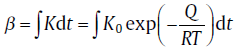 (23)
(23)
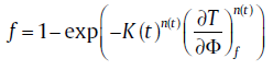
Following the assumption of randomly dispersed nuclei growing isotropically, the relationship between f and β (i.e., Eq. (22)) can be specified as[8, 9, 10, 11, 12, 13]
f=1-exp(-β n) (24)
If an extreme nucleation mode (i.e., site saturation or continuous nucleation) and interface-controlled growth mode hold, substituting Eq. (23) into Eq. (24) leads to the classical KJMA (Eq. (18)) or KJMA-like (Eq. (19(a)) and (19(b))) model, respectively, for isothermal and isochronal cases. Therefore, the equations of state for the degree of transformation are identical for the case of isothermal and isochronal annealing if they are expressed in terms of β .
Prior to that, the “ KJMA-like” theory is defined specifically for the case of non-isothermal transformation. In a more general sense, this term should include various modifications of the original KJMA equation, such as the diffusion-controlled growth (m = 2), anisotropic growth (Eq. (15(b))) and the non-randomly dispersed nuclei (Eq. (15(c))), considering the essential philosophy of the KJMA (-like) model follows the assumptions that the transformation mechanism remains unchanged while the kinetic parameters are assumed to be constant with respect to time and temperature throughout the temperature/time range of interest.
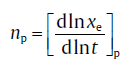
It is often observed from the kinetic analysis that the kinetic parameters vary with the progress of transformation, which is traditionally interpreted as corresponding changes in the nucleation and growth mechanisms during transformation. But the recently proposed analytical model[13] provides a more reasonable explanation. Summation/product transition (SPT) is essential for the derivation of this analytical model[29],
 (25)
(25)
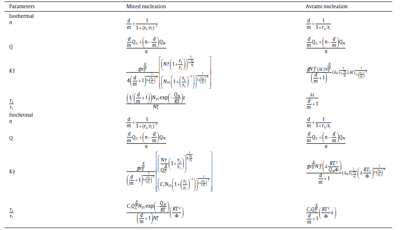
where xe1 and xe2 are the extended transformed fractions due to pure site saturation and pure continuous nucleation, r1, 2 (=xe2/xe1) is an important parameter to characterize the relative contributions of two sub-processes. The analytical model consists of three mechanisms, i.e. nucleation, growth and impingement of growing new-phase particles, and is applicable to both isothermal and isochronal transformations. By choosing suitable nucleation and growth modes, in particular a mixed nucleation mode, the model leads to analytical formulations for the degree of transformation which exhibit a framework of the KJMA-like equation (Eqs. (20) and (21)) but with variable kinetic parameters (see Table 2). The kinetic analysis for solid-state phase transformations is carried forward by this effective model; see the following sections.
| Table.2 Expressions for the growth exponent, n, the overall activation energy, Q, and the pre-exponential factor of rate constant, K0, to be inserted in analytical model for isothermal annealing and isochronal annealing, respectively. Results are given for mixed nucleation and Avrami nucleation |
In traditional kinetic analysis, many concise recipes have been adopted for the determination of the kinetics parameters, such as Avrami plot (isothermal)[7] and Ozawa plot (isochronal)[30] for identifying the Avrami exponent, and Kissinger (-like) plot[31, 32] or isoconversion method[33, 34, 35] for determining the overall effective activation energy. Even though these recipes, based on the classical KJMA (-like) model, were proposed for the transformation with constant kinetic parameters, it has been proved, in terms of analytical model, that they are valid for the transformation with variable kinetic parameters (see Reference 14). Furthermore, because the analytical model can provide more specific kinetic information, several kinetic analysis recipes were proposed accordingly.
For transformations with mixed nucleation (or Avrami nucleation), there are two parts contributing to the overall extended transformed fraction: one due to pure site saturation and the other due to pure continuous nucleation. The relative contributions of the two parts decide the prevailing mode, i.e., the ratio between the extended transformed fraction due to site saturation and that due to continuous nucleation depends on which nucleation (Avarami or mixed one) occurs. In addition, the growth mode defines the variation range of kinetic parameters. These typical features can be reflected by the evolution of kinetic parameters, and recipes for determination of nucleation and growth modes were proposed as a consequence.
For isothermal transformation, the Avrami plot can be expressed as[7, 14]
 (26)
(26)
And the activation energy can be obtained from[7, 14]
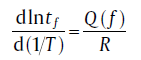 (27)
(27)
with tf representing the time needed to attain a fixed f at different isothermal annealing temperatures. The two equations lead to the evolution of kinetic parameters with transformed fraction, which are totally different for the transformations controlled by mixed nucleation and Avrami nucleation, i.e., for mixed nucleation, n increases with f, and for Avrami nucleation, n decreases with f. The range of n values between d/m andd/m+1 indicates the growth mode and dimension. In addition, the evolution of Q with fcan be regarded as strong evidence of the determined nucleation mode.
For isochronal transformation, a conversion from a continuous cooling or heating transformation (CCT/CHT) into an isothermal transformation (TTT) should be performed first. Recently, an approach to describe the CCT (CHT)-TTT conversion has been proposed by using additive rule[36]:
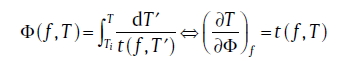 (28)
(28)
On this basis, the transformed fraction of isochronal transformation can be expressed as[37]
 (29)
(29)
After conversion, the prevailing modes of nucleation and growth in the isochronal transformation can be determined by the outcome of the converted isothermal transformation, because the nucleation and growth modes remain unchanged upon the CCT (CHT)-TTT conversion.
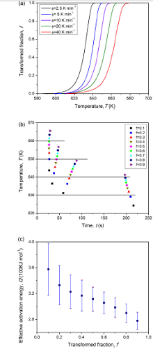
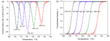
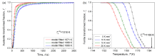
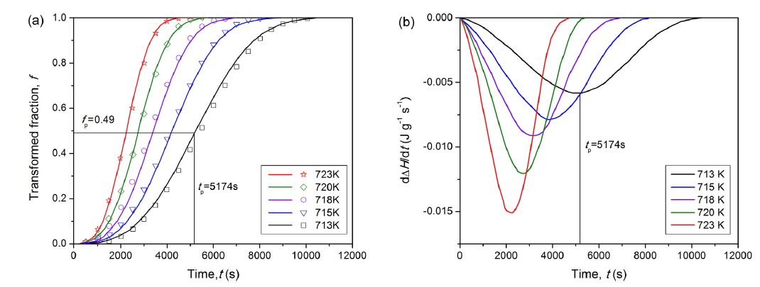
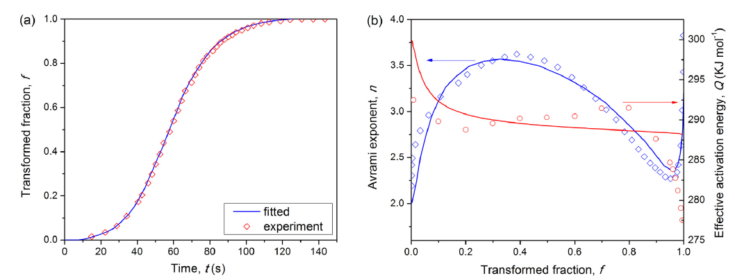
The above procedure has been applied to the isochronal crystallization of pre-annealed amorphous Pd40Cu30P20Ni10 alloy[38]. The evolution of transformed fraction calculated from the isothermal DSC curves is shown in Fig.4(a). Accordingly, a conversion of CHT-TTT was performed, thus giving a series of isothermal transformations (see Fig.4(b)). Applying Eq. (26), the range of n between 1.0 and 2.2 indicates a diffusion-controlled growth occurring upon the crystallization. Fig.4(c) plotted from Eq. (27) exhibits a decreasing Q with f, which implies that mixed nucleation occurs within the crystallization. The successful application of the analysis procedure suggests that it is an effective tool for the determination of transformation mechanisms.
 | Fig.4 (a) Transformed fraction as a function of temperature, due to isochronal crystallization of amorphous Pd40Cu30P20Ni10 after pre-annealing for 100 s at 626 K; (b) TTT diagram conversion using the additive rule (Eq. (26)); and (c) the effective activation energy as a function of transformed fraction[38]. |
The experimental data at a maximum transformation rate measured by DSC were often adopted in traditional kinetic analysis, for example, the DSC peak temperature was adopted in the Kissinger plot[31]. However, the kinetic information obtained from maximum transformation rate data is very limited by the traditional recipes. The revisiting of the maximum transformation rate on the basis of analytical model will extract much more crucial kinetic parameters[39]. The following part illustrates the recipes for identifying the Avrami exponent, the activation energies for nucleation and growth, and the impingement mode from maximum transformation rate analysis.
For isothermal transformation, values at the maximum transformation rate obey the following formulas[39]:for impingement due to random nuclei dispersion
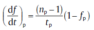 (30a)
(30a)
for impingement due to anisotropic growth
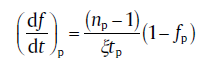 (30b)
(30b)
and for impingement due to non-random nuclei dispersion
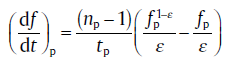 (30c)
(30c)
The subscript p denotes the values at the peak. Application of Eq. (30(a)), (30(b)) and (30(c)) leads to infinite numbers of np and impingement factor (ξ or ε ). Meanwhile, the relationship between np and impingement factor should also obey the following equation[14]
 (31)
(31)
In combination with this constraint function, a unique set of np and impingement factor can be identified.
For isochronal transformation, the impingement factor depends directly on the value of f at the maximum transformation rate, fp[39] value can be calculated as follows:for impingement due to random nuclei dispersion
fp=1-e-1(32a)
for impingement due to anisotropic growth
fp=1-ξ 1/(1-ξ ) (32b)
and for impingement due to non-random nuclei dispersion
ε (fp)ε -1 xe|f=fp =1(32c)
With the impingement factor obtained from Eq. (32(a)), (32(b)) and (32(c)), the values fornp can be further determined by[40]
where the values for Qp can be derived by the Kissinger plot.
In terms of the analytical model, it gives[39]:for isothermal case
lng1=ln(1/tp (1/(np-d/m)-1))=C1-QN/RTp(34a)
for isochronal case
lng2=ln(RTp/Φ (1/(np-d/m)-1))=C2+QN/RTp(34b)
By plotting lng1 (or lng2) with 1/RTp, the value for QN can be obtained from the slope. In combination with np, Qp and QN, the value for QG can be determined by
 (35)
(35)
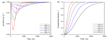
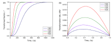
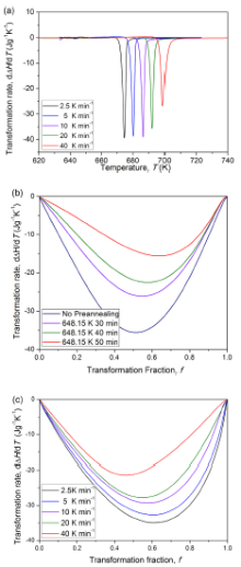
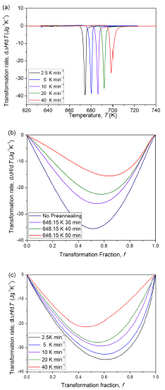
Application of the maximum transformation rate analysis identifies the impingement mode and the values for n, Q and QN and QG. This recipe has been applied to experimental data on the isothermal crystallization of pre-annealed amorphous Mg80Cu10Y10 alloy[39]. The evolution of transformation rate and transformed fraction measured by DSC are shown inFig.5. Using the transformation rate maximum data from Fig.5 and applying Eqs. (30(a)), (30(b)) and (30(c)) and (31) yield np
 | Fig.5 Experimental values for (a) rate of enthalpy change and (b) transformed fraction as a function of transformation time, for the case of isothermal crystallization of pre-annealed (at T= 428.2 K for 3600 s) amorphous Mg80Cu10Y10 as measured by DSC at the temperatures indicated[39]. |
In the previous part, the maximum transformation rate analysis was used to extract some crucial kinetic information. However, there are still two limitations in this recipe, i.e., the procedure to determine the impingement mode of isothermal transformation is rather complicated, and the determined value for QG changes within a range. On this basis, more effective recipes have been proposed correspondingly.
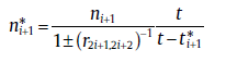
An iterative method was proposed to identify the impingement factor of isothermal transformation. In the literature, the classical KJMA model was often expressed as the normalized form for the sake of simplicity[42, 43, 44]. It has been proved that the normalized treatment is compatible with the analytical model[45]. Traditionally, the normalized treatment was performed with a randomly selected time. Recently, it has been found that the normalized form includes the impingement information if a characteristic time, t* , is selected. The transformed fraction at a characteristic time, f* , varies with the impingement mode [45]:
for impingement due to random nuclei dispersion
f* =1-e-1(36a)
for impingement due to anisotropic growth
f* =1-ξ 1/(1-ξ ) (36b)
and for impingement due to non-random nuclei dispersion
 (36c)
(36c)
Based on Eq. (36(a)), (36(b)) and (36(c)), the iteration approach was proposed for the determination of impingement factors. A randomly selected value is first set as the initial f* , and an initial impingement factor can thus be calculated from Eq. (36(a)), (36(b)) and (36(c)). Then, the experimental data can be used to examine precisely the initial value. If the model prediction, using the calculated impingement factor, agrees with the experimental data very well, the calculated impingement factor can be regarded as true value. Otherwise, another value for f* is selected to replace the initial value and to repeat the previous steps. Compared with tedious error-trial approach applied in the maximum transformation rate analysis, the new method will identify the value for impingement factor after several simple iterations. This method has been applied to the isothermal crystallization of Cu46Zr45Al7Y2 bulk metallic glass[45]. According to the crystallized fraction and crystallization rate of this alloy (see Fig.6), the iteration procedure in combination with Eq. (36(a)), (36(b)) and (36(c)) leads to the impingement mode, i.e., the crystallization conducted at different temperatures is due to weak anisotropic growth (ξ = 1.4634, 1.5185, 1.3703 and 1.2586, respectively, for T= 738, 743, 748 and 753 K).
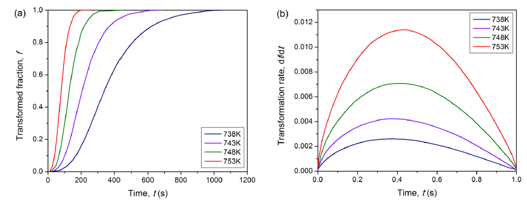 | Fig.6 Experimental values for (a) transformed fraction as a function of transformation time and (b) transformation rate as a function of transformed fraction for the case of isothermal crystallization of Cu46Zr45Al7Y2 bulk metallic glass as measured by DSC at the temperatures indicated[45]. |
Based on the evolution of kinetic parameters as a function of f, a concise recipe was proposed for determining the exact values for QN and QG. According to the analytical model, the relationship between Q and n can be rewritten as [46]
 (37)
(37)
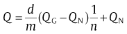
The values for d/m and n(f) and Q(f) can be obtained from the traditional analyzing recipes. A linear relationship between 1/n and Q can be plotted via f. Accordingly, the values for QG and QN can thus be obtained from the linear regression analysis.
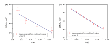
This recipe has been examined by the numerically calculated transformations, which suggests that it is more concise and reliable than the commonly used methods for the determination of QN and QG. According to the values for n and Q determined by the traditional recipes, the nucleation and growth activation energies of the crystallization of many amorphous alloys have been determined by the linear regression analysis, i.e., for Zr55Cu30Al10Ni5 alloy (see Fig.7(a)), QN = 172 ± 8 kJ mol-1 and QG = 379 ± 8 kJ mol-1; and for Zr50Al10Ni40 alloy (see Fig.7(b)), QN
 | Fig.7 Plotting the overall activation energy against the reciprocal of Avrami exponent: (a) for the isothermal crystallization of Cu46Zr45Al7Y2 bulk amorphous alloy and (b) for the isothermal crystallization of Zr50Al10Ni40 bulk amorphous alloy[46]. |
Without recourse to any kinetic model, the kinetic analysis recipes were applied to extract the kinetic information directly; see the previous section. Determining exact parameter values and identifying transformation mechanisms require much more elaborate analysis based on model fitting. For example, a huge body of literature exists on fitting the classical KJMA (-like) model to the experimental data, e.g. crystallization of amorphous alloys. However, such fitting procedure leads only to phenomenological explanation for many transformations because of the limitations as mentioned in Section 1. Recently, the analytical model used to fit the experimental data yields reasonable results. Furthermore, the analytical model has been modified in order to describe more general transformations. This section discusses recent development in application and modification of analytical model.
Using different nucleation, growth and impingement modes as shown in Section 3, researchers constructed various transformation mechanisms in terms of modular analytical model[14]. For any mechanism, the transformed fraction can be calculated by model prediction. The least squares difference between the model prediction and the experimental data was minimized using a fitting procedure by altering the values for the model parameters. The goodness of the fits was calculated as the sum of the absolute differences between fitted values and experimental ones. Thus, the values of kinetic parameters and transformation mechanisms correspond to the fitted results with optimum goodness of the fits[47].
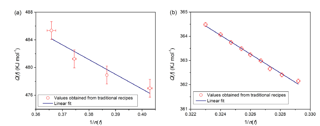
The crystallization kinetics of bulk amorphous Pd40Cu30P20Ni10 alloy was investigated by recording isothermal (or isochronal) DSC scans at different temperatures (or heating rates)[48]. Subsequent analysis of the experimental data produces the transformation rates of isothermal and isochronal annealing of amorphous samples without pre-annealing treatment. Considering the nucleation and growth modes, researchers fit the following analytical models to the measured transformation rate curves: (A) mixed nucleation and interface-controlled growth, (B) Avrami nucleation and interface-controlled growth, (C) mixed nucleation and diffusion-controlled growth, and (D) Avrami nucleation and diffusion-controlled growth. The model parameters are determined by fitting the analytical model, i.e., A-D, to the experimental data as obtained for either various holding temperatures (i.e., isothermal annealing experiments) or various heating rates (i.e., isochronal annealing experiments), simultaneously.
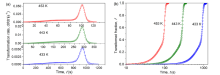
For the isothermal crystallization of Pd40Cu30P20Ni10 without pre-annealing, the analytical models based on interface-controlled growth, i.e., A and B, gave a better fit (seeFig.8(a)), in contrast with models based on the diffusion-controlled growth. This is satisfactorily compatible with the star-like, radially growing product microstructure as observed by SEM, which is ascribed to the result of eutectic growth[8]. It cannot be excluded that a good fit may be established by more than one combination of values of these parameters. The most “ reasonable” fit should provide a minimum error and physically realistic values for the fit parameters. Recognizing that same values have been obtained for the goodness of fit in both A and B models, determining which model, A or B, provides the preferred description requires further analysis. The analysis of model parameters suggests that the isothermal crystallization of Pd40Cu30P20Ni10 complies with model B: interface-controlled growth and Avrami nucleation.
 | Fig.8 Rate of enthalpy change due to (a) isothermal and (b) isochronal crystallization of amorphous Pd40Cu30P20Ni10 as measured (symbols) and as fitted (lines), by assuming mixed nucleation (solid lines) or Avrami nucleation (dashed lines)[48]. |
For the isochronal crystallization of Pd40Cu30P20Ni10 with or without pre-annealing, the models based on diffusion-controlled growth (C and D models) provide better fits to the experimental data (see Fig.8(b)), in contrast with models based on interface-controlled growth. This corresponds to particles precipitating in a matrix and with a composition different from that of the matrix (cf, the SEM observations in Reference 8). Further discussion of the values obtained for the model parameters concludes that both nucleation mechanisms, i.e., mixed nucleation and Avrami nucleation, in combination with diffusion-controlled growth, provide a satisfactory description of isochronal crystallization of Pd40Cu30P20Ni10.
Indeed, the direct fitting procedure described in Section 5.1 can identify the transformation mechanisms and determine the values of kinetic parameters exactly. However, there are some drawbacks in this procedure, for example, more than one set of reasonable fitted results yields. In view of this, researchers have recently proposed a new method[49] which provides a straightforward route for the determination of reliable values of kinetic parameters.
To choose reasonable initial values of the kinetic parameters in the model used for fitting to the full transformation rate curves, a pre-selection of possible operating nucleation, growth and impingement modes should be made by transformation-rate maximum analysis[49]. Thus, the newly proposed procedures for the determination of kinetic parameters are as follows: (i) Select the prevailing mode of impingement and determine the value of np by transformation-rate maximum analysis. (ii) Infer starting proposals for the prevailing nucleation and growth modes. (iii) Choose values for v0, N0/N* , QN and QG. (iv) Perform full transformation curve fitting, based on the pre-selected nucleation, growth and impingement modes. The fit with the least errors provides the optimal results for kinetic parameters. (v) Repeat these procedures for different modes of nucleation and growth to select the prevailing modes by the lowest errors for the fit.
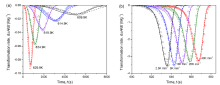
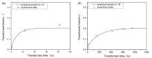
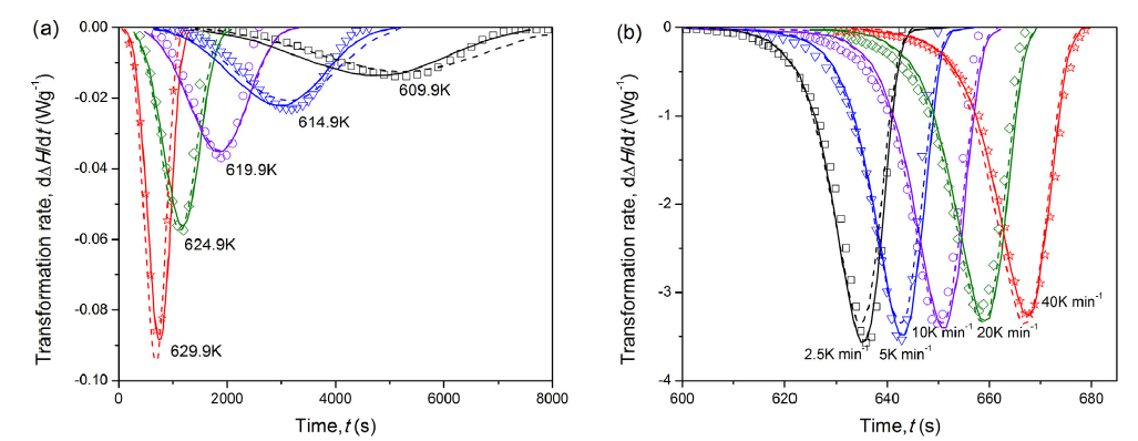
These procedures have been applied to the crystallization of amorphous Zr50Al10Ni40alloy[49]. The evolution of crystallization rate and crystallized fraction with time for the isothermal crystallization of pre-annealed specimens are shown in Fig.9(a) and 9(b). The transformation-rate maximum analysis is first performed on the specimen pre-annealed atT= 713 K, of which the required maximum data are marked in Fig.9(a, b). Eqs. (30(a)), (30(b)) and (30(c)) and (31) yield that the crystallization of pre-annealed specimens follows to a large extent site saturation, three-dimensional interface-controlled growth (i.e., np = 3.06) and random nuclei dispersion impingement. Applying the same maximum analysis to specimens pre-annealed at other annealing temperatures leads to the same conclusion. Further, Eq. (27) yields the activation energy, i.e., Qp = QG = 390 kJ mol-1. Adopting the above analysis results, the crystallization of the pre-annealed specimens can be described as Eq. (19(b)). Then, fitting Eq. (19(b)) simultaneously to all isothermal transformation runs yields a good fit by setting reasonable initial values for v0 and N (seeFig.9(b)). The isothermal and isochronal crystallization of the specimens without pre-annealing have also been described successfully in the same way.
 | Fig.9 Evolution of transformed fraction with time for the isothermal crystallization of (a) pre-annealed and (b) as-quenched Zr50Al10Ni40 amorphous alloy; as measured (symbols) and as fitted (lines) in combination with the maximum transformation rate analysis[49]. |
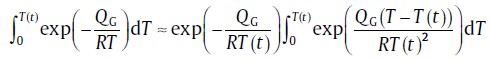
For isochronal transformation, to derive analytical expression for xe, it is inevitable to encounter “ temperature integration” or “ general temperature integration” , which cannot be integrated analytically. During the derivation of the analytical model, the two integration terms roughly approximated, and the lower limit of the integration is considered to be 0 for the sake of simplification[13]. Such approximations make the model concise, but deviate significantly from the exact values when the initial temperature, T0, is high and/or the overall activation energy is small. For this, the model is modified to give more exact analytical expressions.
In the literature, several more accurate approximations for “ temperature integration” and “ general temperature integration” have been proposed, respectively[50, 51, 52]:
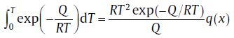 (38a)
(38a)
and
 (38b)
(38b)
where x represents Q/RT and M is a constant, q(x) and p(x, M) are rational equations ofx and/or M[53]. By incorporating the effect of T0 and adopting Eq. (38(a)) and (38(b)), the modified analytical model[53] has the same form as Eq. (21), but with different expressions for the kinetic parameters.
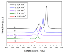
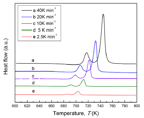
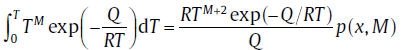
The isochronal DSC curves of amorphous crystallization of Ti50Cu42Ni8 alloy show a two-stage crystallization peak[54] (see Fig.10). The initial temperature of the second crystallization peak approximates the ending temperature of the previous one. This implies that the value of T0 is so high that the modified model has to be applied. Applying the transformation-rate maximum analysis, the impingement mode is identified as randomly dispersed nuclei and isotropic growth. On this basis, the modified model with optimized combination of approximations for temperature integral is fitted to the experimental DSC curves[55]. The fitting results are in good agreement with experimental data (see Fig.11).
 | Fig.11 Evolution of (a) transformation rate and (b) transformed fraction with temperature for the second isochronal crystallization peak of Ti50Cu42Ni8 amorphous alloy; as measured (symbols) and as fitted (lines) by model incorporating the effect of initial temperature[55]. |
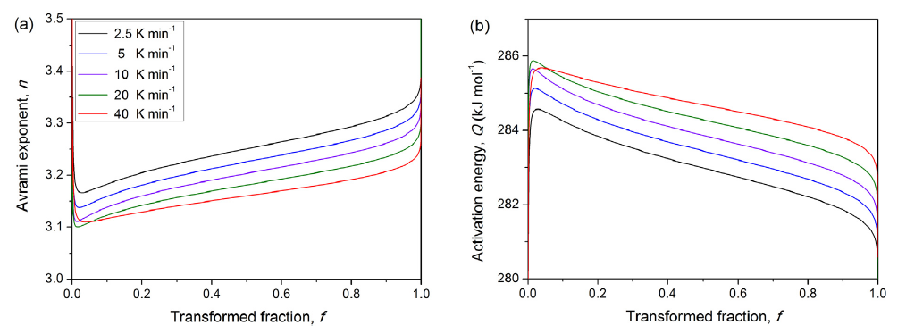
Substituting the fitted parameters, the evolutions of kinetic parameters are shown inFig.12. As can be seen, the increasing n between 3 and 4 indicates that the crystallization mechanism is controlled by mixed nucleation and interface-controlled growth, which corresponds to the eutectic reaction during the second crystallization stage of Ti50Cu42Ni8 amorphous alloy. In addition, compared with the activation energies for self-diffusion in pure metal[56], the calculated Q values exist in a reasonable range. In short, the modified model describes the isochronal crystallization of the amorphous Ti50Cu42Ni8alloy very well.
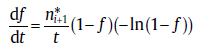
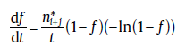
It is generally known that the isochronal kinetic behavior is strongly influenced by the transient effect[57, 58]. However, this kinetic phenomenon is excluded from the derivation of the original analytical model. Recently, the analytical model is modified by incorporating the transient effect, and the expression for this case can be expressed as[59],
 (39)
(39)
where the transient effect is coupled into ψ ; for its specific expression (see Reference59). In terms of the new model, kinetic analysis recipes are modified correspondingly (see below).
By incorporating the transient effect, the transformed fraction corresponding to the maximum transformation rate, fp, derives from the following equations [59]:
 (40)
(40)
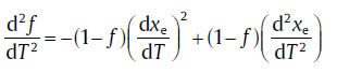
At the transformation-rate maximum, d2f/dT2 = 0 holds. Combining Eqs. (39) and (40), it leads to the expression for (xe)p[59]:
 (41)
(41)
where subscript p denotes the peak values. Following that, fp can be calculated viafp=1-exp(-(xe)p).
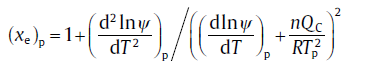
In the traditional method, the values for n can be determined by Eq. (33) for isochronal case. Whereas, Eq. (33), with consideration of the transient effect, should be modified as[59]:
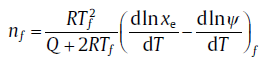 (42)
(42)
where subscript f denotes the values at a fixed transformed fraction. The transient effect is represented by the term dlnψ /dT, which brings n a reasonable value.
Traditionally, the activation energy is often acquired by the Kissinger plot (Eq. (25)). And for the modified model, Q can be obtained in a similar way with transient effect incorporated. Taking logarithm on both sides of Eq. (39), then[59]
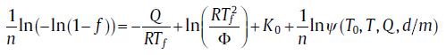 (43)
(43)
To obtain Q from Eq. (43), an iterative method should be adopted by selecting proper initial values of T0 and Q (for details, see Reference 59).
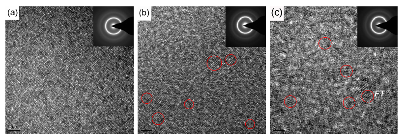
This model was used to study the crystallization behavior of amorphous Fe40Ni40P14B6alloy[59]. From isochronal DSC curve of as-quenched specimens (see Fig.13(a)), the transformation-rate maximum deviates from the “ fingerprint” value (i.e., fp = 0.632), which is attributed to transient effect. For the pre-annealed and fluxed specimens (see Fig.13(b, c)), it was found that both fluxing and pre-annealing processes alleviate the transient effect. This can be explained by the atomic-scale structure observed from the high resolution transmission electron microscopy (see Fig.14): both pre-annealing and fluxing promote the relaxation of the system close to the meta-stable equilibrium state, and atomic-level structure becomes more similar to the corresponding crystallized phase, leading transient effect to be insignificant.
 | Fig.13 (a) Isochronal DSC scans for as-quenched Fe40Ni40P14B6 amorphous alloy; evolution of the rate of enthalpy change with transformed fraction for (b) pre-annealed and (c) fluxed Fe40Ni40P14B6amorphous alloy[59]. |
In applying the SPT in analytical model (see Section 3.4), it is assumed that the site saturation and continuous nucleation contribute to the overall extended transformed fraction, both of which contribute to an accumulation of new phase. Actually, in many transformations, the mechanisms are more complicated than this assumption; for example, multi-processes (more than two) with different nucleation and growth modes occur synchronously or asynchronously. In order to describe these more general transformations, the analytical model is extended[29].
The SPT was firstly extended to the transformation involving two reverse processes: a positive one contributing to the accumulation of new phase and a negative one consuming new phase. The original (i.e., Eq. (25)) and extended SPT can thus be given in a compact form[29]:
 (44)
(44)
where the symbol “ ± ” adopts plus and minus, respectively, for two positive and two reverse sub-processes. By comparison with the rewritten KJMA kinetics, i.e., Eq. (20), the expressions for kinetic parameters are given as
 (45a)
(45a)
 (45b)
(45b)
 (45c)
(45c)
with n* , Q* and K0* as the overall kinetic parameters (for r1, 2, see Section 3.4). From Eq. (45(a)), it can be concluded that the increasing and decreasing trends in Avrami exponent are attributed to the parallel and reverse sub-processes, respectively.
In practice, an assumption of transformation involving two sub-processes is extremely simple, as compared to a combination of various sub-processes. For a transformation involving i (> 2) synchronous sub-processes (each sub-process with constant kinetic parameters, nz, Qz and K0z), xe can be expressed as[29]
 (46)
(46)
where xez represents the absolute value of extended transformed fraction due to sub-process z. According to Eq. (44), Eq. (46) can be rewritten as[29]
 (47)
(47)
where nz* , Qz* and K0z* represent the kinetic parameters after z (=1, 2, 3…) times SPT. Since the SPT is mathematically strict regardless of the variable kinetic parameters, the SPT can be applied to Eq. (47) further. It is found that the expression for xe will reduce one term after each SPT. Therefore, after i-1 times SPT, the summation form of transformed fraction in Eq. (46) can be expressed as a product form[29]:
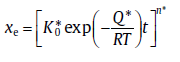 (48)
(48)
Note that there is a recursive relation among the kinetic parameters after each SPT, and the overall kinetic parameters are given in terms of the sub-process kinetic parameters.
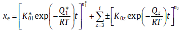
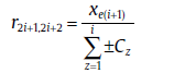
There are also many transformations involving various times asynchronous sub-processes. The physical process of such cases is very complicated. If the transformation mechanisms remain unchanged within a certain range, its kinetics can be specifically modeled. For this case, xe can be expressed as [29]
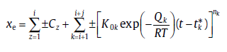 (49)
(49)
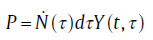
where the first and the second terms on the right represent the extended transformed fraction due to the whole contribution or consumption of i ended sub-processes and of jactive sub-processes, respectively, tk* is the starting time of sub-process k. In this case, the SPT is used to derive the rate equation. If only one sub-process is prevailing within the range, i.e., j = 1, the transformation rate can be given as [29]
 (50)
(50)
with
 (51a)
(51a)
 (51b)
(51b)
Similarly, for the transformation with j (≥ 2) active sub-processes in the range, SPT will lead to the rate equation [29]:
 (52)
(52)
with
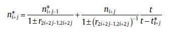 (53a)
(53a)
 (53b)
(53b)
Eq. (50) has the same form as the classical rate equation but with variable Avrami exponent, n* . Due to the variation of mechanisms at critical time, the overall Avrami exponent can never reflect the nucleation and growth modes. Fortunately, the recursive relation between the overall and the sub-process kinetic parameters still hold (see Eq.(53(a)) and (53(b))), which can be used to identify the specific transformation mechanisms.
The current model has been used to explain many interesting kinetic phenomena: the transformation mechanism subject to Avrami nucleation can be regarded as a combination of various time synchronous sub-processes; a process due to continuous nucleation can be regarded as the total effect of infinitely many sub-processes due to site saturation starting at different critical points, etc. Furthermore, this model is an effective tool for describing the multi-peak transformations, (e.g., the isothermal crystallization of amorphous Mg65Cu25Y10 alloy shown in Fig.15) and abnormal isochronal transformations (e.g., the isochronal crystallization of amorphous Zr46Cu46Al8 alloy shown in Fig.16)[29].
 | Fig.15 Evolution of (a) transformation rate and (b) transformed fraction with time for the isothermal crystallization of amorphous Mg65Cu25Y10 alloy; as measured (symbols) and as fitted (lines) by time asynchronous kinetic model[29]. |
The soft impingement and anisotropic growth which break the assumptions of the classical KJMA theory often occur in real transformation. Using the statistical treatment, researchers have specifically addressed the effects of these two kinetic phenomena. This section discusses the recent developments based on the modular analytical model.
6.1.1. Two-stage model
Soft impingement has been found to prevail in several kinds of solid-state phase transformations, e.g., primary crystallization and precipitation[56]. Because the overlapping of concentration field leads to growth rate varying with transformed fraction, this factor was neglected in the originally analytical model, where a constant growth rate is assumed. Recently, by assuming a site saturation nucleation and a linear concentration gradient in front of the growing interface, a physically realistic analytical model incorporating soft impingement for isothermal solid-state precipitation has been proposed[60].
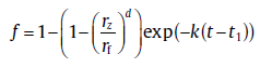
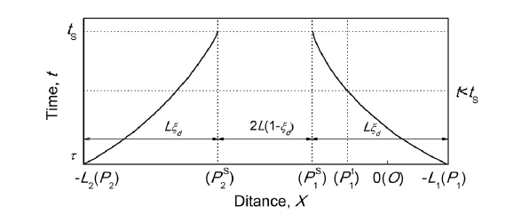
The soft impingement process can be schematically illustrated in Fig.17, where precipitation is divided into two stages. In the first stage, the size of precipitated particle, rI, is smaller than the critical size, rz, and the growth rate of particle, which is not influenced by the neighboring grains, obeys Eq. (16). According to the classical treatment by Zener, rI is expressed as [24]
rI=λ d (D(t-τ ))1/2(54)
where λ d, a function of the pertinent concentrations, is defined as the growth coefficient; τ , the incubation time. Taking the final size of precipitated particle, rf, as a reference, the transformed fraction during parabolic growth is given as[60]
 (55)
(55)
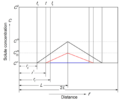 | Fig.17 Schematic diagram depicting a soft impingement process, i.e., a linear approximation for the concentration profile in front of the interface, and a transition from non-overlapping to overlapping diffusion fields[60]. |
In the second stage, r is larger than rz, giving overlapping diffusion fields and in turn retarding growth rate. For this case, the steps for describing the kinetics are shown as follows. First, according to the linear-gradient approximation and the conservation law of mass, the critical size of soft impingement is given as [60]
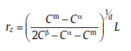 (56)
(56)
with 2L as a distance between two growing particles, Cm a saturated composition in a single-phase alloy before transformation, Cβ and Cα the equilibrium solute concentration of the product phase and the parent phase after transformation, respectively. Then, assuming the starting time for soft impingement as t1, the evolution of Cm is related to time after t1[60]:
Cm (t)=Cα -(Cα -Cm)exp(-k1 (t-t1)) (57)
where k1 = 2D(Cβ - Cα )2/((Cβ - Cm)L)2 for one-dimensional case, and k1 = 12B1D(Cβ - Cα )2/((Cβ - Cm)L)2 with B1 as a rational function of rI/L for three-dimensional case. Finally, substitution of Eq. (57) into Eq. (56) presents an evolution of f with t during soft impingement as [60]
 (58)
(58)
where k = (dD/2)(λ d/rf)d(D(t1- τ ))(d- 2)/2(1 - (rz/rf)d)-1. Note that the present model is expressed in a compact form for the one-dimensional and three-dimensional precipitations, i.e., for d = 1 and d = 3. Therefore, the model should be used with great caution when describing two-dimensional precipitation.
Then, a compact expression for the evolution of transformed fraction yields[60]
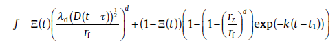 (59)
(59)
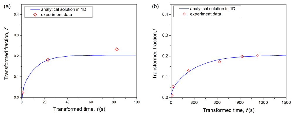
where Ξ (t) = 1, if T< t1; Ξ (t) = 0, if T> t1. Such compact form implies that the current model essentially provides a clear picture for a transition from non-overlapping to overlapping diffusion fields of the growing neighboring precipitates. Note that following the same basic assumptions, the soft impingement model is extended to the isochronal precipitation[61]. On the basis of this model, the method for determining the activation energy of precipitation has been proposed[62, 63]. Good agreement with published experimental data has been achieved by applying this model to real precipitation processes (examples are shown in Fig.18).
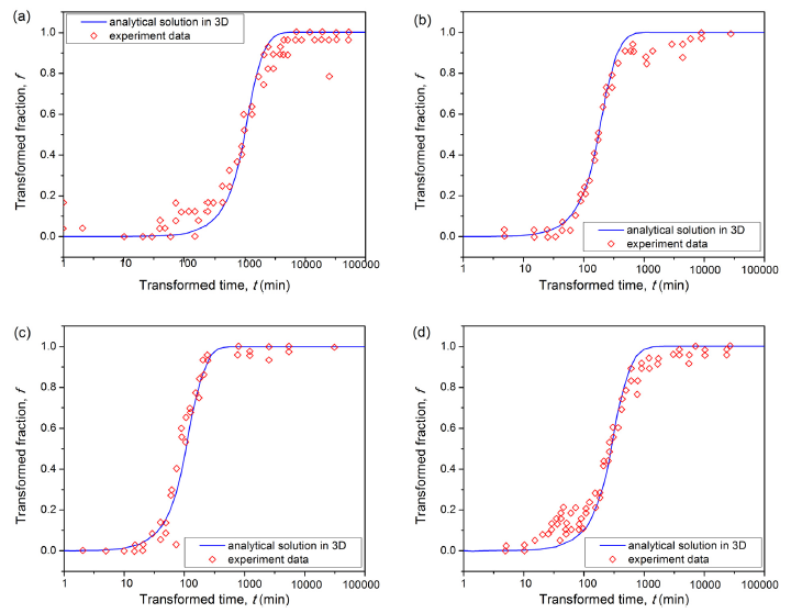 | Fig.18 Evolution of transformed fraction with time in isothermal precipitation of Al-0.2wt%Sc alloy at different annealing temperatures: (a) 503 K, (b) 543 K, (c) 603 K, and (d) 643 K[60]. |
6.1.2. Application of statistical treatment
The treatment in previous section is the so-called geometrical model, which accounts for geometrical distribution of the transformed phase and the surrounding stabilized parent regions, and performs a simplified local mass balance of a growing grain. This section discusses an alternative method of statistical treatment[64], which can be applied to describe the overall kinetics of diffusion-controlled transformations assuming site saturation or continuous nucleation.
First, the case assuming site saturation is considered. Fig.19 shows the probability of an arbitrary point O (X = 0) being transformed by the growth of grain 1 nucleated at P1 (X = L1), subjected to the influence of grain 2 nucleated at P2 (X = -L2)[64]:
dΩ S=2(N* dL1)(N* dL2)exp[-N* (L1+L2)] (60)
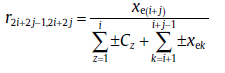
where the factor, 2, indicates that the point O can be transformed by the growth of both grain 1 and 2, N* dL1 and N* dL2 are the probabilities of forming nuclei at P1 and P2 of length dL1 and dL2, respectively, the exponential term is the probability that no nucleus exists in the whole region between P1 and P2. As expressed in Section 6.1.1, the precipitation is divided into two stages. Accordingly, Eq. (60) is integrated in each stage, in combination with a linear approximation of the concentration gradient, a mass balance of solute atoms moving from β phase to α phase, and a conservation law of mass at the interface. The results are given as [64]
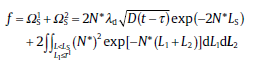 (61)
(61)
where and are, respectively, the parts of f without and with soft impingement, λ d calculated by the probabilistic method has the same expression with that of geometric model, and Ls is the sum length of grain and its diffusion field.
 | Fig.19. Schematic diagram for statistical treatment of diffusion-controlled transformations assuming site saturation[64]. Herein, |
Then, the case of continuous nucleation is considered by using a similar method. The main difference between the continuous nucleation and site saturation is nucleation time. In continuous nucleation, the two nuclei form at two different times, τ 1 and τ 2, respectively. Applying the statistical treatment, f is also expressed by the two parts [64]:
 (62)
(62)
where the expressions for
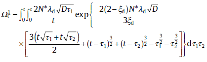 (63)
(63)
with ξ d as the degree of supersaturation, whereas
Compared with various models depending on the degree of supersaturation, this model can be considered the first analytical model that does not depend on supersaturation. Therefore it can be applied without any restriction of supersaturation. In the first stage where soft impingement does not happen, the present model can be reduced to the geometric model. The results of numerical calculation of geometrical model and present model suggest that the two models coincide very well in the early stage. This model is also adopted to describe the kinetics of isothermal austenite-ferrite transformation in 0.37C-1.45Mn-0.11V microalloyed steel (Fig.20)[64], and a good agreement between the model predictions and the experiment results is achieved. Note that the present model leads to the analytical expression only in combination with one-dimensional growth, thus it can only be employed to describe one-dimensional problem. In 0.37C-1.45Mn-0.11V microalloyed steel, the ferrite grows both along the boundaries and into the austenite grains; the growth of the grain boundary involves the movement of a planar ferrite/austenite interface and the growth rate of allotriomorphs is controlled by carbon diffusion in the austenite located before the interface. This problem can be approximately considered a one-dimensional problem. Thus the present model is applicable.
In the analytical model, a phenomenological extension of the original KJMA formulation is used to deal with the anisotropic effect, i.e., Eq. (17(b)). This approach changes only the relation between f and xe, but does not change xe itself. Actually, according to the physical essence of anisotropic growth, the blocking effect will reduce xe[65]. Therefore, a statistical analysis for the blocking effect arising from the anisotropic growth has been performed[66].
In terms of probability, the derivation of the KJMA equation depends on probability that a randomly chosen point in space (e.g., the origin point O) will have remained untransformed at a given time t. The probability that a particle nucleated at time τ will grow to the origin point O when t was expressed as [66]
 (64)
(64)
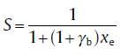
This probability corresponds to the differential form of extended transformed fraction, dxe(see Eq. (18)). Once the blocking effect is included, a non-blocking probability, S(t), should be introduced [66]:
P=S(t)dxe(65)
where S(t) represents all the orientation-, time- and position-averaged values of the non-blocking probability factors. As illustrated in Fig.21, a statistical treatment of the blocking effect is proposed. A particle nucleating at and growing anisotropically toward the origin by a rate dY can be considered an isotropically growing particle with invariable volume. As the transformation proceeds, the growing particle is progressively interfered by different scales blocking. Accordingly, one time blocking decreases the volume increment by 1 - γ b times, with γ b as the non-blocking factor. Thus, the core issue of studying the anisotropic effect becomes the derivation of the probability functions for a particle encountering k-scale blocking.
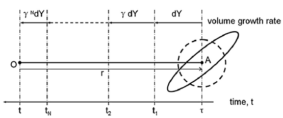 | Fig.21 Schematic diagram depicting a statistical treatment of the blocking effect arising from the anisotropically growing particles. The broken circle indicates that an anisotropically growing particle is equivalently considered as an isotropically growing particle with invariable volume[66]. |
For particles subjected to infinite-scale blocking, the probability is calculated as[66]
 (66)
(66)
According to Eq. (66), the transformed fraction accounting for the infinite-scale blocking which arises from the anisotropic growth is expressed as[66]
 (67)
(67)
Note that this equation is exactly the same as the phenomenological Eq. (17(b)) with ξ = 1 - γ b (0 < γ b < 1). This strongly shows that the phenomenological treatment corresponds just to the extreme case where the particle encounters infinite-scale blocking. In real transformations, the finite-scale blocking often appears. Using the same philosophy, the transformed fraction accounting for the k-scale blocking arising from the anisotropic growth can still be obtained.
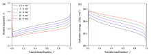
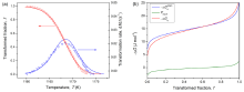
Applying this model to the isothermal crystallization of amorphous Fe33Zr67 alloy (Fig.22(a))[66], researchers have concluded that the Avrami exponent, subjected to the anisotropic effect, changes as a function of the transformed fraction, whereas the effective activation energy is not affected by the anisotropic effect (see Fig.22(b)). Fitting the new models to this transformation, good agreement between the model prediction and experiment data is achieved (see Fig.22).
 | Fig.22 Evaluation of (a) transformed fraction and (b) kinetic parameters for the isothermal crystallization of Fe33Zr67 amorphous alloy; as measured (symbols) and as fitted (lines)[66]. |
Furthermore, the interaction between anisotropic growth and soft impingement during diffusion-controlled phase transformation has been investigated as well. On this basis, the effects of the anisotropic and soft impingement effect in retarding the transformation are further evaluated from the evolution of Avrami exponent[67].
During derivation of the analytical model, it is assumed that the thermodynamic state of system is basically invariant during the whole transformation, the effect of thermodynamics on the transformation kinetics is marginal, and the kinetic equation obeys the Arrhenius equation[14]. This is exactly the case for the transformation occurring in the extremely non-equilibrium state, e.g., amorphous crystallization. However, it becomes invalid for the transformation in the near-equilibrium regime, e.g., austenite(γ )/ferrite(α ) transformation. In order to describe the transformation in the near-equilibrium regime, the analytical model is modified by coupling the thermodynamic energy terms.
In γ /α transformations, the nucleation and growth rates are controlled by both thermodynamic terms (e.g., the critical energy barrier for nucleation and the driving force for growth) and kinetic terms (e.g., activation energies for nucleation and growth) [22, 68, 69]. In order to obtain the exact expression for transformed fraction, Eqs. (4) and(12) have to be used. In this case, the chemical driving force, Δ Gchem, is incorporated into the kinetic equation to obtain the extended analytical model[21].
During the model derivation, an improved treatment is applied for the “ temperature integral” approximation[70]:
 (68)
(68)
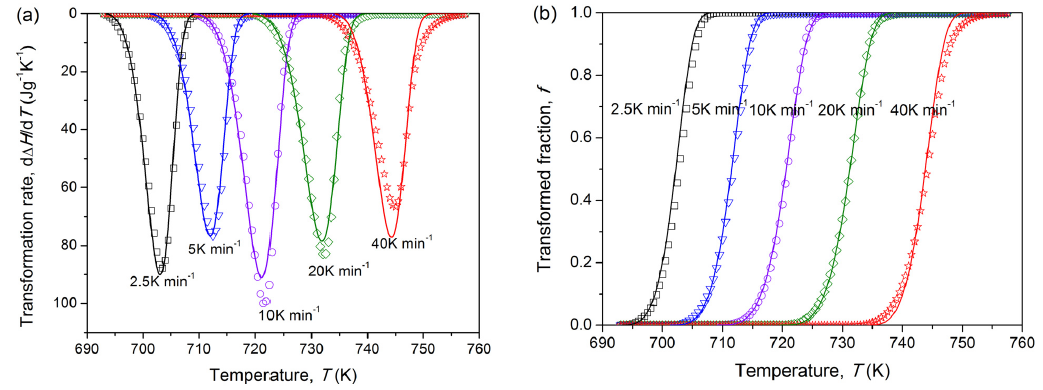
After performing some treatment, it leads to the same equation as Eq. (21) but with K0varying with temperature[21]:for continuous nucleation
equation
 (69)
(69)
for site saturation
 (70)
(70)
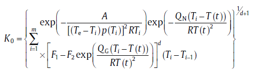
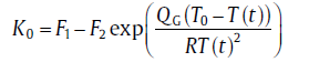
where F1 and F2 are the functions of temperature; for their specific expressions, see Reference 21. Accordingly, the general isochronal rate equation can be obtained[21]:
 (71)
(71)
where H is a differential form of K0. In this model, the effects of the thermodynamic term and kinetic term distinguish explicitly. The kinetic term has the same form as the classical model, e.g., the Avrami exponent: n = d+ 1 for continuous nucleation or n = dfor site saturation; the overall effective activation energy: Q = [dQG + (n- d)QN]/n, whereas the effect of thermodynamic term is included in K0 and H. Therefore, K0 does not follow the ordinary sense of pre-exponential factor of the rate constant. In addition, no specific assumption between T0 and T has been made during the derivation, so the extended analytical model can be applied to the case of either continuous heating or cooling.
With the extended analytical model, the validity of the traditional analysis recipes based on Arrhenius equation has been tested for the transformations occurring in the near-equilibrium state. Due to the effect of thermodynamic terms, the result of traditional recipes (e.g., Kissinger and Friedman methods) for the determination of overall activation energy is H times of its real values. Since the value of H deviates significantly from unit in the near-equilibrium state, the traditional recipes become invalid. Accordingly, several new recipes based on the extended analytical model have been proposed [71-72].
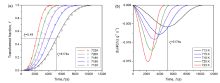
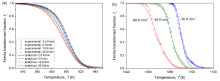
The extended model has been applied successfully to describe the overall kinetic behavior of the γ /α transformations in Fe-3.28 at.% Mn and Fe-1.67 at.% Cu alloys [21](see Fig.23). As compared to the previous works where a site saturation assumption was generally made, the prevalence of continuous nucleation deduced using the extended analytical model prediction gave more reasonable explanation.
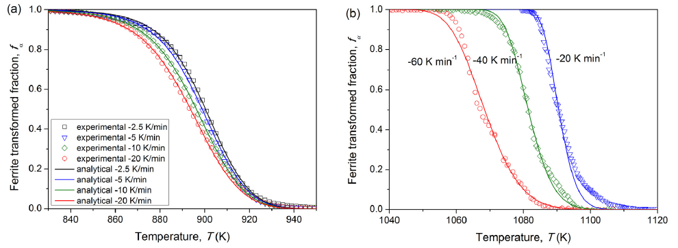 | Fig.23 (a) Evolution of ferrite fraction with temperature for the isochronal austenite to ferrite transformation in (a) Fe-3.28 at.% Mn and (b) Fe-1.67 at.% Cu alloys[21]. |
Figure options
It is generally acknowledged that the misfit accommodation energy plays an important role in the kinetics of solid-state phase transformation. A reliable correct estimation of the total misfit accommodation energy and mechanical driving force is indispensable. Many factors influence this thermodynamic term, whose precise description is a great challenge[73, 74]. On the basis of spherical inclusion, infinitesimal deformation theory, and displacement continuity at the interphase, the interaction between elastic-plastic misfit accommodation and phase transformation is analyzed[75].
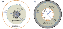
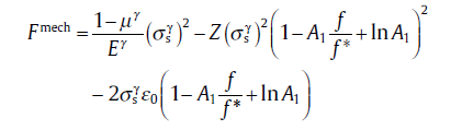
Consider a growing (or shrinking) spherical inclusion subjected to an inelastic volume dilatation and imbedded in a finite, concentric, spherical elastic-plastic matrix which is stress-free at the external surface (see Fig.24)[75]. Taking the γ /α transformation of Fe-based alloy as example, at the initial and the later stages of transformation, the ferrite and the austenite were recognized as the spherical inclusion, respectively, and a sphere packing factor f = f* was introduced to distinguish the two stages. In addition, another two critical transition states further divide these two stages, i.e., f = f1 (or f = f2) at which the outer boundary of the plastic shell within the austenite (or ferrite) matrix overlaps with the matrix boundary. The transformation misfit will induce the elastic and plastic zones around matrix-inclusion interface. With the progress of transformation, the elastic and plastic zones continuously change, which results in the evolutions of accommodation energy with transformed fraction. Corresponding displacement, stress and strain fields have been constructed by using the equation group such as Hooke's law, equilibrium equation, geometric equation and yield criterion and the constraint conditions such as displacement continuity at interphase, pure elastic volume strain and appropriate boundary conditions. And the evolution of mechanic driving force, Fmech, derived analytically[75]for 0 ≤ f ≤ f1,
 (72a)
(72a)
for f1 ≤ f ≤ f* ,
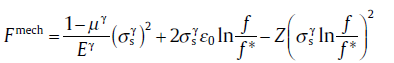 (72b)
(72b)
for f* ≤ f ≤ f2,
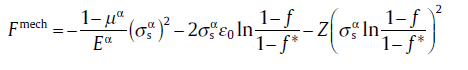 (72c)
(72c)
for f2 ≤ f ≤ 1,
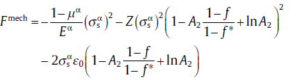 (72d)
(72d)
with µ as the Poisson ratio, E the Young's modulus, σ s the normal stress, ε 0 the misfit strain, 
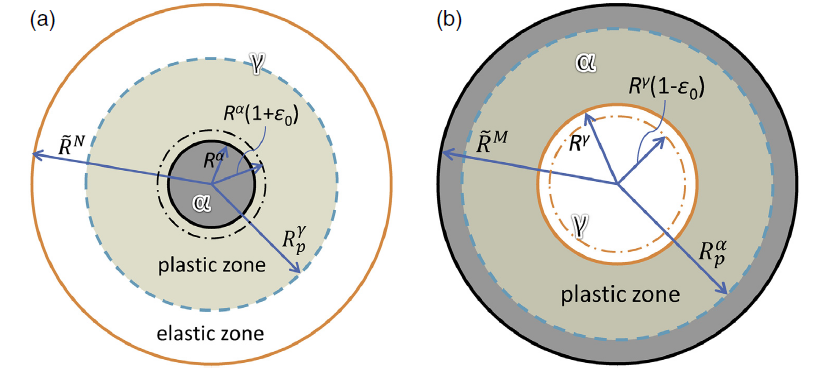 | Fig.24. Schematic diagram depicting a misfitting spherical inclusion growing or shrinking in a concentric elastic-plastic spherical matrix: (a) the ferrite as the inclusion growing in the austenite matrix and (b) the austenite as the inclusion shrinking in the ferrite matrix[75]. Herein, Rα or Rγ , |
Then, by incorporating the mechanic driving force, the growth rate used in analytical model should be revised[75] as
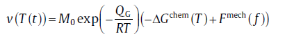 (73)
(73)
Here, the mobility data of the γ /α phase interface were adopted. The exactness of this parameter has a significant impact on the predicted model results. For example, in the recent kinetic studies on the γ to α phase transformation of substitutional Fe-based alloys[27], the mobility data of α /α grain boundaries for the recrystallization of pure iron were used instead of the γ /α phase interface; thus, an abnormal high value for Fmech was obtained. According to the present model, it suggested that the mobility data evaluated by Hillert and Hö glund[68] are a reasonable one. By replacing Eq. (12) with this equation, the analytical model can be used to describe the transformation influenced significantly by the misfit accommodation. This model has been evaluated by using the γ /α transformation of pure iron. The evolution of accommodation implies that the elastic strain energy is much smaller than plastic work so that it can be neglected, matrix is always in a completely plastic state during almost the entire transformation process, and Fmech varies monotonously with f, which counteracts transformation at initial stage but favors transformation at later stage.
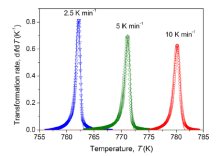
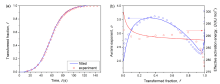
The effect of the misfit accommodation on γ to α transformation kinetics of pure iron has been investigated [75]. The measured isochronal γ to α transformation rate and phase fraction of pure iron with average grain size of 273 µ m upon cooling at a rate of 10 K min-1are shown in Fig.25(a). Using the mechanical driving force model with the material properties, the evolution of the mechanical driving force was calculated (see Fig.25(b)). Based on the thermodynamic assessment, the evolutions of chemical driving force and total driving force are also shown in Fig.25(b). In combination with total driving force, this model was applied to fit the experimentally obtained f and df/dt, simultaneously, and good agreements were achieved (see Fig.25(a)).
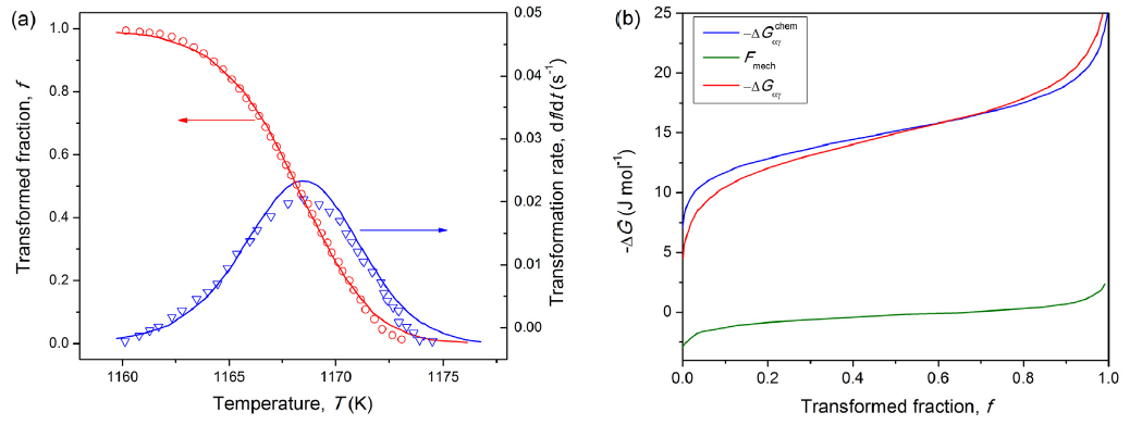 | Fig.25 (a) Evolution of transformed fraction (red line and symbol) and transformation rate (blue line and symbol) with temperature for the isochronal austenite to ferrite transformation in pure iron; as measured (symbols) and as fitted (lines); (b) evolution of the components of driving forces for transformation[75]. |
Since different thermodynamic factors vary in different ways with the progress of transformation, the competition between the thermodynamic terms varying with temperature and transformed fraction has been investigated[76]. This theory provided more reasonable explanation for many interesting kinetic phenomena in the near-equilibrium regime, such as, uncompleted isothermal transformation[77], retarding isothermal transformation behavior at the end stage[78, 79] and abnormal isochronal transformation kinetics[80]. In the following, this theory is briefly discussed.
The thermodynamic and kinetic conditions for the isothermal annealing were evaluated first. The net driving force, Δ Gnet, often contains two parts: the negative one Δ Gchem, which favors the transformation, and the positive one Fmech, which counteracts the transformation, i.e., Δ GneT= Δ Gchem+ Fmech. The driving force is dissipated by migrating interface in two ways: solute drag, Δ Gdiff, and interface friction, Δ Gfri[81]. Based on the solute drag theory, the diffusion of substitutional atom inside the interface and in the spike in front of the migrating interface dissipates Gibbs energy greatly. This term can be expressed as[81]
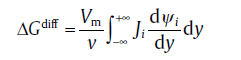 (74)
(74)
where Vm is the molar volume, v the interface velocity, Ji the diffusional fluxes and ψ ithe diffusion potential of i atom, y the distance from the interface. Meanwhile, the Gibbs energy dissipation due to the interface friction is expressed as
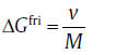 (75)
(75)
The transformation will stop when the net driving force is insufficient for balancing the Gibbs energy dissipation in the near-equilibrium state. Therefore, a thermodynamic state must be met to drive the transformation[76]:
Δ Gfri=-Δ Gchem-Fmech-Δ Gdiff> 0(76)
Meanwhile, the kinetic condition requires that the transformed fraction arising from the inevitable continuous heating/cooling stage (before the isothermal annealing stage) be negligible. Defining a critical transformed fraction, fc, the kinetic condition was expressed as [76]
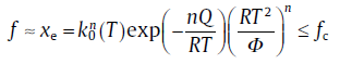 (77)
(77)
According to Eqs.[76, 77], two critical temperatures can derive from the two conditions.
The role of thermodynamic and kinetic conditions can be demonstrated by the simulated transformations (see Fig.26). For the case of Fig.26(a), the thermodynamic condition is violated, so the isothermal transformation cannot be completed even after a sufficiently long time. For the case of Fig.26(c), a noticeable transformed fraction occurs upon previous cooling stage because of the unsatisfied kinetic condition. And for the intermediate case (see Fig.26(b)), both of the above two phenomena occur because the thermodynamic and kinetic conditions are violated simultaneously. Therefore, in order to complete an isothermal transformation, these two conditions have to be satisfied simultaneously.
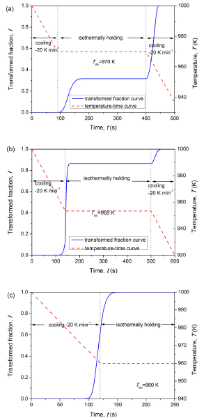 | Fig.26 Numerically calculated transformed fraction as function of time during cooling process interrupted at various isothermally holding temperatures (Tiso): (a) 960 K, (b) 953 K, and (c) 950 K[76]. |
When the complete transformation is observed, the overall kinetics can be described by a recently proposed thermo-kinetic model by coupling the influence of different thermodynamic terms. The model has the same form as the classical rate equation, but with a K0 varying with temperature and transformed fraction[76]:for site saturation,
K0={gN* M0d d[-Δ Gchem-Fmech-Δ Gdiff]}1/n(78)
for the isothermal case of continuous nucleation,
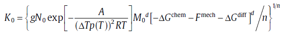 (79a)
(79a)
and for the isochronal case of continuous nucleation,
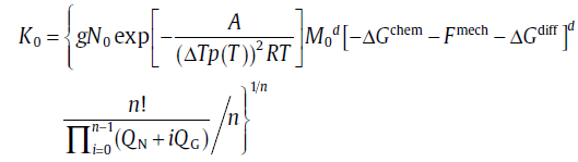 (79b)
(79b)
According to the new model, Fmech accumulates upon isothermal transformation, but other thermodynamic terms remain unchanged, which results in a continuous decrease of net driving force, and thus the sluggish transformation rate in late stage. The abnormal isochronal transformation kinetics is well explained by this model, i.e., the competition between Δ Gchem and Fmech results in the several transformation stages. During the initial stage, compared with Δ Gchem, Fmech is so small that the transformation conducts at a relatively high rate. With the progress of transformation, the accumulated Fmech will restrict the transformation rate. If the transformation conducts continuously to a large degree, the accumulating rate of Fmech slows down, and a relatively high transformation rate is obtained again.
The isothermal and isochronal γ /α transformations are carried out in two binary substitutional Fe-based alloys (i.e. Fe-3.28 at.% Mn and Fe-1.73 at.% Co) [76]. During the interrupted heating process, the complete isothermal α to γ transformation in Fe-3.28 at.% Mn was measured for three holding temperatures (see Fig.27(a)). By fitting the thermo-kinetic model to the transformed fraction as shown in Fig.27(a), the fitted parameter can be used to calculate the evolution of Fmech, which accumulates with the progress of transformation, and in turn leads to the retarded behavior at the late stage. The kinetics of the non-isothermal isochronal γ /α transformations in Fe-1.73 at.% Co are also measured, and the evaluations of ferrite fraction at different cooling rate are shown inFig.27(b). The abnormal kinetics is observed in this transformation, which can be predicted very well by the present model. During this transformation, the fitted values give the values for Fmech, which is large enough to cause the abnormal kinetics.
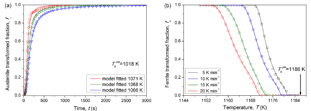 | Fig.27 (a) Evolution of austenite fraction with time for the isothermal ferrite to austenite transformation in Fe-3.28 at.% Mn alloys; (b) evolution of ferrite fraction with temperature for the isochronal austenite to ferrite transformation in Fe-1.73 at.% Co alloys; as measured (symbols) and as fitted (lines)[76]. Herein,  is temperature, when the chemical Gibbs energy of ferrite is equal to that of austenite. is temperature, when the chemical Gibbs energy of ferrite is equal to that of austenite. |
The present review paper illustrates that the analytical model has been widely applied in the field of solid-state phase transformation. Based on the analytical model, several effective kinetic recipes have been developed for identifying the specific transformation mechanisms and determining the values for crucial kinetic parameters, e.g., the maximum transformation rate analysis, the iterative method and the linear regression recipe, which suggests that the analytical model is a flexible kinetic model. In terms of the analytical model, the crystallization kinetics of amorphous alloys with rather complicated mechanisms has been described very well, e.g., the transformation with high T0 and/or lowQ, the transformation influenced by the transient effect and the transformation involving multi-processes, indicating that the analytical model is a general kinetic model. Furthermore, the analytical model takes many factors into consideration, e.g., the soft impingement, the anisotropic growth, and the thermodynamic factors, which implies that the analytical model should be an open kinetic model.
With this useful tool, further study of the kinetic behavior should contribute to the basic physics of solid-state phase transformation. There are two major research directions for the kinetic theory of solid-state phase transformation: the extension of pure kinetics and the correlation between thermodynamics and kinetics. Specifically, for the first category, even when the knowledge on pure kinetics has accumulated over the years, the basic conception of “ iso-kinetics” is still ill-considered; so far, no analytical model has been proposed for describing the transformation with mixed growth mode, and moreover, the interactions between non-randomly dispersed nucleation and anisotropic growth has not been illustrated explicitly. For the second category, it is becoming increasingly clear that both the thermodynamic condition and the kinetic process vary with the transformation progress, leading to a growing awareness of an intrinsic relation between the thermodynamic driving force and the kinetic energy barrier. As compared to the first research direction, the second one is a completely promising field full of opportunities and challenges. For example, if a quantitative relationship between thermodynamics and kinetics can be built in the future, at least three targets can be achieved, i.e. (1) phase transformation kinetics involving structure evolution (composition, fraction, chemical potential, morphology, etc.), (2) a unified treatment for diffusional transformation and shear (or diffusionless) transformation, and (3) a quantitative relation among thermodynamic driving force, kinetic barrier and structure evolution. All of these will be carried out in our future work.
The authors are grateful to the financial support of the National Basic Research Program of China (No. 2011CB610403), the National Natural Science Foundation of China (Nos.51134011 and 51431008), the Fundamental Research Fund of Northwestern Polytechnical University (No. JC20120223), and the China National Funds for Distinguished Young Scientists (No. 51125002).
The authors have declared that no competing interests exist.
| [1] |
|
| [2] |
|
| [3] |
|
| [4] |
|
| [5] |
|
| [6] |
|
| [7] |
|
| [8] |
|
| [9] |
|
| [10] |
|
| [11] |
|
| [12] |
|
| [13] |
|
| [14] |
|
| [15] |
|
| [16] |
|
| [17] |
|
| [18] |
|
| [19] |
|
| [20] |
|
| [21] |
|
| [22] |
|
| [23] |
|
| [24] |
|
| [25] |
|
| [26] |
|
| [27] |
|
| [28] |
|
| [29] |
|
| [30] |
|
| [31] |
|
| [32] |
|
| [33] |
|
| [34] |
|
| [35] |
|
| [36] |
|
| [37] |
|
| [38] |
|
| [39] |
|
| [40] |
|
| [41] |
|
| [42] |
|
| [43] |
|
| [44] |
|
| [45] |
|
| [46] |
|
| [47] |
|
| [48] |
|
| [49] |
|
| [50] |
|
| [51] |
|
| [52] |
|
| [53] |
|
| [54] |
|
| [55] |
|
| [56] |
|
| [57] |
|
| [58] |
|
| [59] |
|
| [60] |
|
| [61] |
|
| [62] |
|
| [63] |
|
| [64] |
|
| [65] |
|
| [66] |
|
| [67] |
|
| [68] |
|
| [69] |
|
| [70] |
|
| [71] |
|
| [72] |
|
| [73] |
|
| [74] |
|
| [75] |
|
| [76] |
|
| [77] |
|
| [78] |
|
| [79] |
|
| [80] |
|
| [81] |
|