Search for articles:
Zhenquan Shen
Corresponding authors:
Received: 2018-09-3
Revised: 2018-11-15
Accepted: 2018-11-26
Online: 2019-07-20
Copyright: 2019 Editorial board of Journal of Materials Science & Technology Copyright reserved, Editorial board of Journal of Materials Science & Technology
More
Abstract
Magnesium alloys have shown great potential for their use in the medical device field, due to the promising biodegradability. However, it remains a challenge to characterize the degradation behavior of the Mg alloys in a quantitative manner. As such, controlling the degradation rate of the Mg alloys as per our needs is still hard, which greatly limits the practical application of the Mg alloys as a degradable biomaterial. This paper discussed a numerical model developed based on the diffusion theory, which can capture the experimental degradation behavior of the Mg alloys precisely. The numerical model is then implemented into a finite element scheme, where the model is calibrated with the data from our previous studies on the corrosion of the as-cast Mg-1Ca and the as-rolled Mg-3Ge binary alloys. The degradation behavior of a pin implant is predicted using the calibrated model to demonstrate the model’s capability. A standard flow is provided in a practical framework for obtaining the degradation behavior of any biomedical Mg alloys. This methodology was further verified via the comparison with enormous available experimental results. Lastly, the material parameters defined in this model were provided as a new kind of material property.
Keywords:
Magnesium alloys have been widely explored as a new kind of biodegradable materials, owing to their great potential for the applications in the medical device field [[1], [2], [3], [4]]. Compared with the Fe-based and Zn-based biodegradable metals, Mg-based biodegradable metals have the unique advantage that magnesium ions positively stimulate osteogenesis leading to new bone formation, which is beneficial to the bone fracture healing [3,5]. Moreover, the mechanical strength of magnesium is close to that of the cortical bones. Therefore, the undesirable stress shielding will be reduced, which helps to lower the concerns on re-fracture or unsatisfactory healing outcome at the fracture site [3,5]. These advantages show the application prospects of Mg-based materials as orthopaedic devices. Apart from orthopaedic devices, Mg-based biodegradable metals are also developed to be used as coronary stents [6].
While the ongoing fundamental research keeps improving our knowledge of the Mg-based biodegradable metals, the study on this material has stepped into the clinical translational perspective [[7], [8], [9]]. The first clinically proven Mg-based biodegradable stent (Magmaris, BIOTRONIK, Berlin, Germany) received the CE mark approval in 2016, allowing the company to begin selling the product in Europe.
Despite the significant progress that has been achieved in recent studies, there still exists a crucial problem for the Mg-based biodegradable implants. These implants generally degrade too fast [1]. For temporary implants, the degradation rate of Mg-based implant should match the recovery process of its surrounding tissues [1]. Various methods including alloying, hot/cold working, as well as surface modification have been applied to improve the degradation performance [[10], [11], [12], [13], [14], [15], [16], [17], [18], [19], [20], [21], [22], [23], [24], [25]]. However, if we re-assess the problem, the key part that currently is most lacking is to understand the underlying corrosion mechanism, and more importantly, to be able to characterize the corrosion behavior in a practical framework.
Various types of corrosion mechanism were reviewed in the Refs. [26,27], including the localized corrosion, galvanic corrosion, stress corrosion cracking, intergranular corrosion, and corrosion fatigue. These mechanisms were summarized based on experimental observations. However, most of the research on the corrosion mechanisms focuses on analyzing the problem at the qualitative level. For adjusting and controlling the degradation rate per our needs, it is imperative to understand the corrosion mechanism in a quantitative manner. Especially, the corrosion rate which indicates the corrosion process with regard to time is a typical index to be formulated. There have been efforts to develop models that are capable of accessing the corrosion rate [[28], [29], [30], [31], [32], [33]]. These models are all based on galvanic corrosion or diffusion mechanism. The common drawback of these models is that they are limited to the micro corrosion theory itself rather than focusing on the actual orthopaedic devices. In other words, these models are still not suitable for being directly used in engineering design or evaluation. Gastaldi et al. [34] and Boland et al. [35] built a phenomenological corrosion damage model (CDM) under the frame of finite element method, which was applicable for orthopaedic devices. The CDM model can be extended to many scenarios including uniform corrosion [34,36], pitting [37], stress corrosion [34,36] and strain corrosion [38]. However, CDM neglects the diffusion process, which is the fundamental physical factor in the corrosion process. Grogan et al. [39] built a physical model taking diffusion into consideration. However, the result from their work deviates from the actual situation. There are no experimental results verifying the model, which makes its correctness doubtful. Besides, it is only applicable to pure magnesium. The model can only predict the degradation process that is less than 1 h. All of these constrains limit the applicability of their model from the perspective of engineering application.
In this paper, a degradation model based on diffusion mechanism is developed and the finite element implementation is presented. After the calibration with in vitro corrosion data, the degradation model presents great consistency with the experimental results. A pin implant is simulated with the established model to demonstrate the capability of this model. Based on this process, a standard flow of obtaining the degradation behavior of Mg-based alloys is then summarized into a practical framework, which combines the FE modeling and in vitro sample test to eventually generate an easy-to-use fitted degradation curve. This methodology provided here is then further verified via the comparison with enormous available experimental results. In the meanwhile, corresponding parameters of these materials which are defined in this model are provided as a new kind of material property. This model is proved to have a great significance on adjusting and controlling degradation rate of Mg-based biodegradable metal implants.
Magnesium and its alloys can gradually corrode in aqueous solutions with hydrogen evolving. At the same time, corrosion products deposit on the surface of bulk material forming a protective layer [40]. Based on the fact that there is a film formed on the surface of the magnesium alloy when it corrodes in vitro or in vivo, the effects of the corrosion layer must be taken into account. As shown in Fig. 1, a simplified model is established, which consists of magnesium alloy, corrosion layer, and corrosion environment. With magnesium alloy gradually degrading, the interface between the solid magnesium alloy and corrosion layer moves toward the alloy. Meanwhile, magnesium ions produced by solid material corrosion diffuse into the aqueous environment across the corrosion layer.
Fig. 1. Schematic diagram of magnesuim alloys corrosion.
According to the Fick’s law, the diffusion is governed by the equation:
where c is the concentration of diffusion ions, D is the diffusivity, t represents time, ∇ denotes the gradient. Referring to the conventional single-species model [30], although the product of corrosion consists not only magnesium ions, the assumption made here is that only magnesium ions are considered diffusing in the corrosive medium.
Scheiner and Hellmich [41] showed that the moving velocity of boundary between corrosion layer and solid magnesium matrix is related to the concentration and diffusivity through equation:
{-D∇cenv-(csol-ccor)v}⋅n=0 (2)
where v is the velocity of the moving boundary, n is the interface normal vector pointing the corrosion layer side. Four parameters directly control the diffusion and boundary moving process, namely the diffusivity D, the concentrations of magnesium ions in solid alloy csol, in corrosion layer ccor, and in corrosion environment cenv.
The concentration of magnesium ions in solid Mg alloy is dependent on the alloy composition to be modelled. The value of the csol can be calculated through the following equation:
csol=$\frac{ρMg·(1-w)}{ M_{Mg}}$ (3)
where ρMg is the density of high pure magnesium, MMg is the molar mass of magnesium element, w is the mass fraction of alloying elements and impurity. The value of the cenv depends on the composition of the corrosive medium.
The morphology and composition of the corrosion layer can be experimentally measured. For example, it can be seen from the previous research that the composition of the corrosion layer is complicated [42]. The corrosion layer is in porous structure, even varying with time. So, it is impossible to calculate the concentration ccor directly. For the same reason, there is no perfect way to measure the concentration ccor experimentally in situ. Here, we provide an alternative approach to solve this problem. Most magnesium alloys produce magnesium hydroxide when corrodes in the liquid medium. By assuming that the corrosion layer is composed of dense magnesium hydroxide, the concentration ccor can be calculated based on magnesium hydroxide and a correction factor ε owing to the existence of pores and other compositions:
ccor=$\frac{(1-ε)ρMg(OH)_{2}}{M_{{Mg(OH)}_{2}}}$ (4)
where ρMg(OH)2 is the density of magnesium hydroxide, $M_{{Mg(OH)}_{2}}$ is the molar mass of magnesium hydroxide, ε is a phenomenological parameter determined by best fit.
As for diffusivity D, it would vary in different mediums, for instance, in the corrosion layer or in the corrosion environment. Considering that the film is as thin as even tens of nanometers [43], this layer is negligible compared to the size of the corrosion environment. For simplicity, the corrosion layer appears absent in our model. In spite of the geometric absence, its influence on the process is still in existence through the concentration ccor and diffusivity D. The parameter ccor appears in Eq. (2) which controls the corrosion rate. As for diffusivity D, it accounts for all the unknown effects not only including corrosion layer in such a way that it is seen as a phenomenological parameter which can be determined by best curve fit. How diffusivity D is affected by those unknown effects can be studied at a smaller scale. In our model, those details are ignored from the perspective of a large phenomenological scale.
The diffusion-based corrosion model can be implemented into the finite element software ABAQUS using the user subroutine UMESHMOTION [44] for 3D structure problem. As mentioned, the challenge in numerically solving the corrosion problem is that the solid-liquid interface moves as the corrosion is progressing, which makes it a moving boundary problem. In this work, the moving boundary problem is solved by the Arbitrary Lagrangian-Eluerian (ALE) adaptive meshing capability in ABAQUS. Details of this method have been discussed in Grogan et al.’s papers [39,45]. Here, a flowchart of the algorithm is illustrated in Fig. 2. All parts in our model are meshed using 3-D linear coupled temperature-displacement reduced integration brick elements (C3D8RT). For the reason that diffusion equantion has the same form comparing to the heat conduction equation, the temperature degree of freedom is used for user-defined parameter c, the concentration. Concentration of solid parts in the model are set to an invariable value as a boundary condition. Although solid parts occupy the volume of Mg alloy, their concentration value is the corrosion layer concentration ccor which can be seen as boundary of solid parts. The alloy concentration csol only appears in Eq. (2). It affects corrosion rate, but has nothing to do with ions diffusion. Concentration of liquid environment is variable during ions diffusing. The symmetry of the samples and devices is used to reduce numerical calculation.
Fig. 2. Flow chart of the ALE adaptive mesh algorithm.
To calibrate the parameters, a finite element model is set up as shown in Fig. 3(a). In experimental testing, the Mg alloy materials are cut into disk-shaped samples with the size of 10 mm × 10 mm × 2 mm according to our previous work [10,42]. Therefore, the geometric model is created to be the same size as the reality. Symmetry is applied to reduce the size and therefore the calculation, resulting in only one-eighth of the sample being simulated. The simulation result will need to be multiplied by eight to get the final value. In Fig. 3(a), the red part represents magnesium alloy with the constant concentration ccor. The blue part represents corrosion environment of which the concentration and its distribution change with time due to Mg ions diffusing. For this particular case that is used for calibration, the corrosion environment is Hanks solution or simulated body fluid (SBF). The green part represents the interface between the two parts mentioned above. All parts are meshed using 3-D linear coupled temperature-displacement reduced integration brick elements (C3D8RT).
Fig. 3. (a) One-eighth finite element model of the disk-shaped sample used in vitro test, blue part represents corroion environment, red part represents magnesium alloy sample, green part is the interface of the two parts. (b) One-eighth finite element model of the cylinder implant pin.
The evolved hydrogen is used to evaluate the corrosion rate of magnesium alloys. According to the chemical reaction:
Mg+2H2O→Mg(OH)2+H2 (5)
The mass loss or volume loss can be calculated through equation:
vhyd=$\frac{Δv·ρMg·M_{{H}_{2}}}{M_{Mg}·ρH_{2}·S}$ (6)
where Δv is the volume loss of the magnesium alloy, vhyd is the volume of released hydrogen in unit area, MH2 is the molar mass of hydrogen, ρH2 is the density of hydrogen, S is the surface area of the magnesium alloy. For the disk-shaped sample we used, and the S can be calculated by:
S=2a2+4ah (7)
where a is the base dimension of the sample, and h is the thick of the sample.
According to the evolved hydrogen, the calibration process is to find the value of D and ε which can make the simulation results fit the experimental results best. The ε value is fixed first, then D is tuned to match the simulation results with the experiments profile. Under the circumstances that no such a D value is found, the value of ε is then adjusted and the above process is then repeated.
After calibration, the finite element model was used to predict the corrosion behavior of as-cast Mg-1Ca alloy and as-rolled Mg-3Ge alloy implant in vivo. Two cylinder-pin models were developed by the similar method introduced in the above section as shown in Fig. 3(b). Mg-1Ca alloy pin has the dimension of 10 mm in length and 2.5 mm in diameter. Mg-3Ge alloy pin has the dimension of 10 mm in length and 2.2 mm in diameter. Taking symmetry into consideration, only one-eighth of the geometry is modeled. The element type being used here is also C3D8RT. Boundary condition is the same as mentioned in section 2.2. The corrosion environment are two cylinders. One has the dimension of 50 mm in length and 12.5 mm in diameter. The other one has the dimension of 50 mm in length and 11 mm in diameter.
The calibration results are shown in Fig. 4(a) and (c). The immersion time refers to the duration when the samples are immersed in the corrosion medium. Two different alloys are simulated here for the calibration, which are Mg-1Ca and Mg-3Ge showed in Fig. 4(a) and (c), respectively. It is shown that the volume of released hydrogen per unit area increases with the immersion time. The scatters are the data from our previous experimental studies [10,42] representing the sample average values, while the lines are plotted from the simulation results. Details of the experimental method can be found in these two papers [10,42]. The model is calibrated by fine tuning the corrosion parameters ε, D to best fit the experimental results as shown in Fig. 4(a) and (c). Parameter w depends on the material which is used and can be given in advance. The values about these two materials are given in Table 2. Other basic parameters are listed in Table 1.
Fig. 4. (a) As-cast Mg-1Ca alloy, the volume of released hydrogen in unit area varies with immersion time. Scatter is the experimental data, lines are simulation results. (b) as-cast Mg-1Ca alloy, the Mg ions concentration with respect to time. The inserted picture on the bottom right is the sampling points which is marked. (c) as-rolled Mg-3Ge alloy, the volume of released hydrogen in unit area varies with immersion time. Scatter is the experimental data, lines are simulation results. (d) as-rolled Mg-3Ge alloy, the Mg ions concentration with respect to time. The inserted picture on the bottom right is the sampling points which is marked.
Table 1 Basic parameters used in the present study.
| ρMg (kg/m3) | 1735 |
|---|---|
| $ρ_{{Mg(OH)}_{2}}$ (kg/m3) | 2360 |
| ρH2 (g/L) | 0.0899 |
| CHanks (mol/L) | 7.375×10⁻⁴ |
| a (mm) | 10 |
| MMg (g/mol) | 24 |
| $M_{{Mg(OH)}_{2}}$ (g/mol) | 58 |
| $M_{{H}_{2}}$ (g/mol) | 2 |
| CSBF (mol/L) | 1.532×10⁻³ |
| h (mm) | 2 |
Table 2 Parameters of Mg-1Ca alloy immersed in SBF solution and Mg-3Ge alloy immersed in Hanks solution derived from best fitting.
| w | ε | D (mm2/h) | |
|---|---|---|---|
| Mg-1Ca | 1.00% | 0.80 | 1.3×10⁻² |
| Mg-3Ge | 3.00% | 0.10 | 1.0×10⁻⁴ |
Two cylinder pins are simulated with the calibrated corrosion parameters of Mg-1Ca and Mg-3Ge alloys. To match with the calibration process, SBF solution is used as the corrosion environment for Mg-1Ca alloy and Hanks solution is used for Mg-3Ge. The respective material parameters for the two kinds of Mg alloys are shown in Table 1, Table 2. The unit system is properly selected to correlate the simulation time to the immersion time. The units of length, concentration and diffusivity are adopted as mm, mol/L and mm2/h, respectively. As a representation, Mg-1Ca is analyzed in the following two paragraphs. Mg-3Ge is similar.
The contour plot in Fig. 5 exhibits the variation of concentration of Mg ion in the corrosion environment at 0, 50, 100, 150, 200 and 250 h after corrosion. Each picture of Fig. 5(a)‒(f) has two parts. The main part in center is the 3D view of the as-cast Mg-1Ca alloy pin in the SBF solution. The inserted picture at bottom left is the cross-section of the pin. Different color corresponds to different concentration of the Mg ions. The red region represents the non-corroded pin. It can be clearly seen that ions gradually diffuse into the environment. It is obvious that diffusion in cross-section is nearly isotropic. Also, as can be found from the 3D view, corrosion has a marked impact in the end. It implies that the diffusion in axial direction is inhomogeneous.
Fig. 5. Contour plots of the corrosion environment concentration at different time: (a) 0, (b) 50 h, (c) 100 h, (d) 150 h, (e) 200 h, (f) 250 h. The main picture in each figure is 3D view of the Mg-1Ca alloy pin, the inserted picture is cross section of the Mg-1Ca alloy pin.
Fig. 6(a) is the morphology feature of the as-cast Mg-1Ca alloy cylinder pin at 0, 50, 100, 150, 200 and 250 h after corrosion. Experimental results are also provided for comparison in Fig. 6(b). Details of experimental method can be found in previous work [10]. It can be found that cross-section dimension reduces nearly uniformly in every direction, while the curvature on both ends significantly changes with time developing in Fig. 6(a). And the end is gradually rounded. The same features are also found in the Fig. 6(b) and the only difference is that the surface of the implant is rough. The reason why rough surface is appeared is that the environment is complicated in a real body of an animal. The implant has experienced many processes not only diffusion corrosion, but also galvanic corrosion, stress corrosion and so on. However, the whole profile is still the same as simulated result. It is evident that the simulated corrosion is homogenous in the cross section, but it is heterogeneous in axial direction. This kind of structure feature just corresponds to the concentration feature mentioned above. It indicates that there must be some relevance between them. A reasonable explanation is that the local high concentration means rapid corrosion. In consequence, the local structure is cut more. This conspicuous structural change may lead to failure. Hence it is just the position where we should focus. This may give some helpful suggestions about structural design of the medical devices. This analysis embodies that computer simulation can assist in structure design. It is part of the value of this paper.
Fig. 6. Morphology feature of the Mg-1Ca alloy pin over time: (a) simulation, (b) experiment.
Fig. 4(a) shows the volume of released hydrogen in unit area of the as-cast Mg-1Ca alloy disk with respect to the simulated corrosion time. As shown in solid line, the profile increases in an exponential way in the first 50 h of corrosion. After 50 h the profile shows a linear relationship with time.
In this model, corrosion is implemented by moving boundary. So such profile of corrosion is believed to be related to the corrosion near the interface. Based on Eq. (2), the concentration gradient is an important factor, which can affect boundary moving velocity. It is just the concentration difference between the solid interface and the environment near the interface that drives the boundary moving. To figure out the reason why the profile is nearly linear after a while corrosion starts, we investigated the concentration of the environment near the interface.
Fig. 4(b) shows the Mg ions concentration of as-cast Mg-1Ca alloy with respect to time. The inserted picture on the bottom right indicates the sampling points which are marked with orange dots. The 23 points are all near to the interface of the cross section. The line plotted is the mean value of these 23 points. It can be found that the concentration increases rapidly then stabilizes. The stable stage just corresponds to the linear stage of the volume of released hydrogen in unit area in terms of time. This implies that it is just the concentration near the interface that affects the corrosion rate. Also, Fig. 4(c) and (d) about the as-rolled Mg-3Ge alloy shows the same variation trend. Because the span of ordinate in Fig. 4(d) is small, the whole range can be regarded as stable stage corresponding to linear relationship in Fig. 4(c). This conclusion inspires us to adjust the concentration near the interface in order to control the corrosion rate. And it also makes this model directly relate to surface modification. The concentration driven mechanism indicates the direction of surface modification that is controlling the concentration of surface magnesium ions. Many surface modification techniques can be explored [1]. Also, the corrosion products covered on the surface can influence the corrosion rate from the perspective of concentration. It inspires us to design a new kind of magnesium alloy, which can generate corrosion product layer with special concentration on the surface during corrosion. By this means, the corrosion rate is controlled per humans’ need. Magnesium ion concentration at the corrosion product layer is a significant reference index for understanding the protection of surface layer.
Due to the complex nature of the problem, the corrosion rate does not have an analytical formula. One could use numerical simulation with FEA to solve the corrosion for any three-dimensional structures. However, the cost is simulation time and computing resources, especially when the corrosion time of interest is at weeks. Here we present a simple way to obtain a compact degradation curve for much longer corrosion time. As shown in Fig. 7, we fit the calculated data from the first 250 h by a power function:
Δv=AtB (8)
Fig. 7. (a) The weight loss of the Mg-1Ca alloy pin with respect to simulating time. Solid line is the resulted from our model, dash line is obtained from power-law fit of the simulation data, bars are in vivo experiment data. (b) enlarged view of the red part in (a). (c) the volume loss of the Mg-3Ge alloy pin with respect to time. Solid line is the result from our model, dash line is obtained from power-law fit of the simulation data, bars are in vivo experiment data. (d) enlarged view of the red part in (c).
where A and B are two empirical parameters. In the case of Mg-1Ca alloy pin immersed in SBF solution, A equals 0.00198, B equals 0.52207. In the case of Mg-3Ge alloy pin immersed in Hanks solution, A equals 0.00011, B equals 0.98172. Corrosion rate can be derived from the Eq. (8):
$\frac{d(Δv)}{dt}$=A∙BtB-1 (9)
Thus, the formula can be used to predict corrosion over longer time span without computer simulation. From Fig. 7 (a) and (c), we observe that the predicted values are close to the experiment values. Experimental results shown on Fig. 7(a) and (c) are from our previous work [10,42]. However, the predictive corrosion rate of as-cast Mg-1Ca alloy is higher than experimental results in the beginning, and slightly lower than experimental results later. The predicted corrosion rate of as-rolled Mg-3Ge alloy is lower than experimental observations. The deviation gradually decreases with increasing time.
The deviation between theoretical prediction and experiment can be explained from the following aspects: materials, processing technique, corrosion environment and boundary condition. For the perspective of materials, the constituent of Mg alloys varies from each other. The second element or impurity may have some effects such as galvanic corrosion. Since galvanic corrosion is not driven by concentration gradient, this effect is not included in our model. In terms of processing technology, different processing produces different microstructure. Microstructure is an important factor to influence corrosion such as crevice corrosion and intergranular corrosion. Microstructure can even affect stress distribution leading to stress corrosion. The most significant aspect is the corrosion environment. Although people endeavor to simulate the physiological environment, there is still a large gap between in vitro and in vivo. The parameters calibrated from in vitro test are directly applied to in vivo simulation, which introduces some error. The effect of boundary condition is also non-negligible. In our model, corrosion environment is set to have five times the length of Mg alloy’s dimensions. Such an environment is big enough for the diffusion of metal ions for our simulations. However, in the actual physiological environment, there is no enough space in each direction. Once ions reach the boundary, the boundary must have an influence on diffusion.
Although the model is for a uniform corrosion, it is easy to be expanded to simulate the pitting corrosion. Here, we provide just one of the methods which can simulate pitting. Because there is much perturbation in the environment, we can set the initial value of the corrosion layer concentration ccor at some points to be different, so that the corrosion layer is heterogeneous in terms of the distribution of the concentration. Once the heterogeneous layer is formed, the corrosion velocities in these points are different from other parts, which generates pitting corrosion.
Combined with in vitro test, the numerical model can be used as a standardization method to determine the degradation rate. Here we provide a practical framework. First, we calibrate the model parameters by means of immersion test of simple geometry samples. Then, we simulate medical device corrosion with the calibrated parameters over a short period of time. Finally, we obtain the corrosion rate formula through best fit of the results from simulation. Thus, we can predict longer time degradation of the medical device we care about without large calculation. This method is practical and reliable to a certain extend in biomedical engineering.
From the methodology perspective of this practical framework, the model parameters are further discussed here. These parameters are obtained from in vitro test. Are they the same as in vivo experiment? The answer is absolutely no. Unfortunately, there is no better choice so far. The in vitro test is developed to replace the in vivo experiment, which is costly and time consuming. For the purpose of predicting the costly in vivo experiment through a simple in vitro test, this method proposed in this work bridges the gap between in vitro and in vivo tests. The accuracy of this method depends on how the in vitro test approximates the in vivo experiment. The only way to solve the parameters problem is looking forward to the development of in vitro test. The closer the in vitro test is to in vivo experiment, the more accurate the calibrated parameters are. Even at present stage of in vitro test, this method is still a good approximation for actual in vivo results in terms of the corrosion rate. And to the authors’ knowledge, this is the first paper which put forward a method predicting degradation rate directly facing engineering application through simple in vitro test in biodegradable metals field.
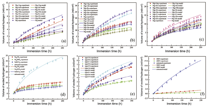
To verify our model in a universal case, we re-analyze the data obtained by other researchers [[46], [47], [48], [49]]. The experimental methods are similar to those for Mg-1Ca and Mg-3Ge. Details can be found in Refs. [[46], [47], [48], [49]]. As shown in Fig. 8, volume of hydrogen evolution varies with immersion time. All the parameter values are listed in Table 3, Table 4, Table 5, Table 6, Table 7. The scatter is experimental data, while the lines are obtained from our simulation. Colors are used to distinguish varieties of alloys and treatments. We can conclude that ε is in relation to degree of crook of the profile. The larger value ε is of, the more curve bends. Meanwhile, D is in relation to the amplitude of the curve. Amplitude will increase with the increase in D value. Also, Mg alloys in SBF have bigger ε values than in Hanks solution. Mg alloys which are treated by surface modification have both bigger values about ε and D in general. Processing technic has no significant influence on D and ε. The most essential discovery is that all these curves follow the power-law approximately.
Fig. 8. Volume of hydrogen evolution varies with immersion time, scatter is experimental data, lines are obtained from our model. (a) as-cast Mg-1X alloys immersed in Hanks solution, (b) as-cast Mg-1X alloys immersed in SBF solution, (c) as-rolled Mg-1X alloys immersed in SBF solution, (d) alkaline heat treated Mg-1Ca alloy immersed in SBF solution, (e) surface modification by chitosan Mg-1Ca alloy immersed in SBF solution, (f) microarc oxidation (MAO) coated Mg-1Ca alloy immersed in Hanks solution.
Table 3 Parameters of as-cast Mg-1X alloys immersed in Hanks solution derived from best fitting.
| w | ε | D (mm2/h) | |
|---|---|---|---|
| Mg | 0.000% | 0.86 | 2.5 × 10⁻³ |
| Mg-1Ag | 0.982% | 0.10 | 9.0 × 10⁻⁵ |
| Mg-1Sn | 0.858% | 0.10 | 7.5 × 10⁻⁵ |
| Mg-1Mn | 0.788% | 0.10 | 7.0 × 10⁻⁵ |
| Mg-1Zr | 0.747% | 0.96 | 4.5 × 10⁻³ |
| Mg-1In | 1.010% | 0.10 | 5.5 × 10⁻⁵ |
| Mg-1Zn | 1.065% | 0.10 | 4.0 × 10⁻⁵ |
| Mg-1Al | 1.162% | 0.10 | 4.0 × 10⁻⁵ |
Table 4 Parameters of as-cast Mg-1X alloys immersed in SBF solution derived from best fitting.
| w | ε | D (mm2/h) | |
|---|---|---|---|
| Mg | 0.000% | 0.10 | 6.5 × 10⁻⁴ |
| Mg-1Mn | 0.788% | 0.20 | 6.8 × 10⁻⁴ |
| Mg-1Ag | 0.982% | 0.80 | 4.8 × 10⁻³ |
| Mg-1Sn | 0.858% | 0.80 | 4.5 × 10⁻³ |
| Mg-1In | 1.010% | 0.90 | 1.2 × 10⁻² |
| Mg-1Al | 1.162% | 0.95 | 3.0 × 10⁻² |
| Mg-1Zn | 1.065% | 0.98 | 1.1 × 10⁻¹ |
Table 5 Parameters of as-rolled Mg-1X alloys immersed in SBF solution derived from best fitting.
| w | ε | D (mm2/h) | |
|---|---|---|---|
| Mg | 0.000% | 0.80 | 3.8 × 10⁻³ |
| Mg-1Sn | 0.858% | 0.80 | 2.7 × 10⁻³ |
| Mg-1Ag | 0.982% | 0.80 | 2.5 × 10⁻³ |
| Mg-1Zr | 0.747% | 0.90 | 6.5 × 10⁻³ |
| Mg-1Si | 1.189% | 0.80 | 2.7 × 10⁻³ |
| Mg-1In | 1.010% | 0.80 | 2.0 × 10⁻³ |
| Mg-1Y | 1.010% | 0.80 | 1.8 × 10⁻³ |
| Mg-1Zn | 1.065% | 0.95 | 1.5 × 10⁻² |
| Mg-1Mn | 0.788%1 | 0.97 | 3.0 × 10⁻² |
Table 6 Parameters of alkaline heat treated Mg-Ca alloy and surface modification by chitosan Mg-Ca alloy immersed in SBF solution derived from best fitting.
| Mg-1.4Ca | ε | D (mm2/h) |
|---|---|---|
| type3-1 | 0.970 | 3.0 × 10⁻² |
| type4-6 | 0.950 | 9.5 × 10⁻³ |
| type1-6 | 0.920 | 4.0 × 10⁻³ |
| type2-6 | 0.900 | 2.5 × 10⁻³ |
| type3-3 | 0.990 | 1.2 × 10⁻¹ |
| type3-9 | 0.970 | 1.0 × 10⁻² |
| type3-6 | 0.990 | 4.5 × 10⁻² |
| Unheated | 0.800 | 1.3 × 10⁻³ |
| Na2CO3 | 0.992 | 6.8 × 10⁻¹ |
| Na2HPO4 | 0.995 | 1.1 |
| NaHCO3 | 0.992 | 2.5 × 10⁻¹ |
Table 7 Parameters of microarc oxidation (MAO) coated Mg-Ca alloy immersed in Hanks solution derived from best fitting.
| Mg-1Ca | ε | D (mm2/h) |
|---|---|---|
| Untreated | 0.0 | 2.5 × 10⁻⁴ |
| MAO 300v | 0.1 | 2.3 × 10⁻⁵ |
| MAO 400v | 0.2 | 1.0 × 10⁻⁵ |
Fig. 8(a)-(c) is the result of the binary Mg alloys. The experimental data of the three figures mentioned above is referred to Gu et al [46]. Good agreement between our model and experiment indicates that our model can be applied to different binary Mg alloys. Comparing Fig. 8(a) with Fig. 8(b), we can draw a conclusion that this model is suitable for both the environments, Hanks solutions and SBF. Besides the initial environment concentration, the composition of corrosion products is also distinct. This leads to the fact that the ε values obtained by best fit are different in the two corrosion environments even if it is the same alloy. Also, the diffusivity D is different from each other in these two solutions. The corrosion environment is one of the effects that can influence the diffusivity D. Comparing Fig. 8(b) with Fig. 8(c), you can see that different wrought process can be reflected in our model. The wrought process has an influence on the diffusivity D and factor ε.
Alkaline heat treated Mg-1Ca alloy is displayed in Fig. 8(d). Experimental data is from Gu et al. [48]. The result reveals that alkaline heat treated can decrease the corrosion rate notably. The values of D and ε change significantly after alkaline heat treatment. According to experimental observation [48], a dense surface formed on the top of Mg-1Ca alloy matrix after alkaline heat treatment and increases the D value.
Surface modification by chitosan on Mg-1Ca alloy is displayed in Fig. 8(e). Experimental data is obtained from Gu et al. [49]. The result illustrates that surface-coated via the parameters D and ε affects corrosion rate in our model.
A microarc oxidation (MAO) coated on a Mg-1Ca alloy is displayed in Fig. 8(f). Experimental data is from Gu et al. [47]. The result declares that MAO coating can decrease the corrosion rate signally. The values of D and ε differ much after MAO treatment. Referring to experimental observation [47], there are a lot of pores on the surface. The higher voltage is, the thicker coated is, and the bigger size pores are of. The value of D decreases with increasing voltage, while the value of ε increases with increasing voltage. In another word, the thickness of coated and size of pores have an influence on the diffusivity D and the factor ε.
On the one side, the discussion in this section is to prove our model has the ability to include a variety of situations through the two parameters D and ε. Moreover, it will be as a beginning to study how these two parameters are affected. We just give a macroscopic preliminary understanding. On the other side, the parameters listed in Table 3, Table 4, Table 5, Table 6, Table 7 are corresponding D and ε of these Mg alloys. As two kinds of material properties, the values are given out in this paper. All in all, Fig. 8 proves that our model has wide applicability in various situation and the power-law is ubiquitous in consideration of magnesium alloy degradation.
A corrosion model of the biomedical Mg alloys has been established based on the underlying physics that covers diffusion process, corrosion layer existence, and surface morphology change. The ALE adaptive meshing and user subroutine UMESHMOTION in ABAQUS have been used to implement our model into finite element scheme. A standardization method to determine the degradation rate has been developed in a practical framework. As an example, pin implants made of Mg-1Ca alloy and Mg-3Ge alloy were predicted by this method and compared with in vivo experiment. Further verification with enormous available data about Mg alloys in vitro test has demonstrated that our model can capture the degradation phenomena accurately and has a broad application. As for material properties, the model parameters’ values are provided. The phenomenological parameters are influenced by many effects, which are deserved to be further studied. Power-law degradation rate has been summarized. The methodology presented in this work will play an essential role in understanding, adjusting and designing medical devices for a proper degradation rate in biomedical engineering.
This work was supported by National Key Research and Development Program of China (Grant No. 2016YFC1102402), National Natural Science Foundation of China (Grant No. 51431002 and 51871004), NSFC/RGC Joint Research Scheme (Grant No. 51661165014), and Peking University Medicine Seed Fund for Interdisciplinary Research (Grant No. BMU2018ME005).
The authors have declared that no competing interests exist.

 WeChat
/
| 〈 |
|
〉 |


